Lecture 1.1: Introduction and Decision Theory

TL;DR

1. Machine learning automates inductive inference: from finitely many examples to a general rule. This only works with an inductive bias (an idea of what we look for) and only if the data contains a signal about the output.
2. Setup: $(X,Y)\sim P$ on $\mathcal{X}\times \mathcal{Y}$. A loss $\ell (x,y,y^{\prime })$ says how expensive an error is. The true risk is $R(f)=E(\ell (X,Y,f(X)))$. The Bayes risk $R^{\ast }={\inf }_{f}R(f)$ is the best possible risk, and a function attaining it is a Bayes classifier $f^{\ast }$.
3. For the 0-1 loss, the Bayes classifier is explicit: $f^{\ast }(x)=1$ iff $\eta (x)=P(Y=1\mid X=x)\ge 1/2$ (Theorem 2). Its error at $x$ is $\min (\eta (x),1-\eta (x))$.
4. Surrogate losses (hinge, squared, exponential, logistic) act on a real scoring function $f$. They have different Bayes predictors $f^{\ast }$, but after thresholding at 0 all of them give the 0-1 Bayes classifier: they are classification-calibrated.
5. For regression with the squared loss, the Bayes predictor is the regression function $\eta (x)=E(Y\mid X=x)$ (Theorem 4), because $E|f(X)-Y{|}^2=E|f(X)-\eta (X){|}^2+E|\eta (X)-Y{|}^2$.
6. Decision theory: priors only, maximum likelihood, maximum a posteriori, and the Bayes decision rule with costs: predict the label with the smallest conditional risk. For two classes: predict 1 iff ${\pi }_1{\ell }_{01}p(x\mid 1)>{\pi }_0{\ell }_{10}p(x\mid 0)$. Decision boundaries are the points where the two weighted curves cross.

Exam relevance

• Real exam, task type “Bayes decision” (4 P): a diagram of class-conditional densities is given. You determine the decision boundaries mathematically for ML, MAP or a cost-sensitive rule, compute the error, and reason backwards: which prior or which cost ratio produces a given boundary. See Reading decision boundaries off a diagram.
• Mock exam, task 3: cost-sensitive Bayes classification on a discrete $X$: $\mu$, $\eta$, the Bayes classifier and its error, the threshold $1/(1+a)$, the smallest prior that flips a decision. See the task on the Bayes classifier.
• Multiple choice: consistency of definitions (Bayes risk vs. Bayes classifier, ML vs. MAP), which loss gives which Bayes predictor.
• Sheet 1, Exercise 2 is the same task type as the exam (three classes, prior and loss from a given rule). Exercise 3 is the $L_2$ proof.

Overview: 1. A very short history of AI and ML, 2. Machine learning as inductive inference, 3. The statistical setup: loss, risk, Bayes classifier, 4. Optimal predictions in closed form (0-1 loss, surrogate losses, $L_2$ loss), 5. Statistical and Bayesian decision theory, 6. Reading decision boundaries off a diagram (exam training).

Introduction

A very short history of AI and ML

Slides 4-23

The lecture starts with a short history (for a longer version, see the introduction of Hardt and Recht, Patterns, Predictions, and Actions).

Decade	What happened
1950s	AI gets “invented” at the Dartmouth Summer Conference (1956). Main paradigm: symbolic AI. Rosenblatt’s perceptron (1957) is the first machine that learns: 400 photosensors, a 20 × 20 pixel image, two classes. Huge optimism (“within ten years a digital computer will be the world’s chess champion”, Simon 1958).
1960s	Symbolic AI, ELIZA (1966) mimics a psychotherapist with pattern matching. Minsky and Papert (1969): a single-layer perceptron can only learn linearly separable functions, for example not XOR, and nobody knows how to train multi-layer perceptrons.
1970s	AI winter (Lighthill Report, 1973). First steps in statistical pattern recognition: kNN, naive Bayes, Bayesian decision theory, learning from few hand-designed features.
1980s	Backpropagation makes multi-layer networks trainable (hand-written digits). Decision trees (ID3).
1990s	Deep Blue beats Kasparov (brute-force search, no learning). Modern ML rises: support vector machines, first generalization bounds (VC dimension).
2000s	ML becomes practical: kernel methods, boosting, random forests and bagging, concentration inequalities and generalization bounds. Spam filtering, recommender systems, bioinformatics. DARPA Grand Challenge (2005), Watson wins Jeopardy (2011).
2010s	Deep neural networks: ImageNet with CNNs and GPUs (2012), AlphaGo (2016), transformers (Vaswani et al., 2017).
2020s	Generative AI for images, audio, text and video. Language and foundation models, coding agents.

Several topics of this course appear here: the perceptron (Lecture 2), the VC dimension (Lecture 3), boosting and bagging (Lecture 6) and deep networks in the overparameterized regime (Lecture 8).

What this lecture is about

Slides 28, 30-32

The lecture is rather theoretical. It tries to make the point why and under which assumptions machine learning works or doesn’t work:

• the statistical setup of machine learning: Bayesian decision theory, convergence, consistency, estimation and approximation error, bias-variance tradeoff
• the fundamental principles that enable machine learning (learning theory, stability, regularization, aggregation), both in the classical and in the overparameterized regime
• learning in the interpolation regime and why and when it works
• practical issues: data, training, validation, benchmarking
• machine learning and society: fairness, discrimination, explainability, legal frameworks

Not covered: basic ML algorithms (see an introductory ML course), unsupervised learning, reinforcement learning, probabilistic learning, online learning, time series, images and language models.

Required: maths for ML (linear algebra, multivariate calculus with gradients and Hessians, probability theory) and some first ML algorithms. Literature: mainly Hardt and Recht (2022) and Shalev-Shwartz and Ben-David (2014), sometimes Bach (2024), Hastie, Tibshirani and Friedman, Mohri, Rostamizadeh and Talwalkar, Hardt’s book on benchmarks, and Devroye, Györfi and Lugosi (1996).

Machine learning as inductive inference

Deduction vs. induction

Slides 35-39

Deductive inference

Reasoning from one or more general statements (premises) to a logically certain conclusion. If the premises are correct, all conclusions are correct as well.

Example: every person in this room is a student, every student is older than 10 years, so every person in this room is older than 10 years. Mathematics is built on deduction. But deduction has no natural way to deal with uncertainty about the premises.

Inductive inference

Reasoning that constructs or evaluates general propositions derived from specific examples. The conclusion can always be wrong.

Example: in all our experiments, dropped things fall downwards, so we conclude that things always fall downwards. Humans draw such uncertain conclusions from limited experience all the time.

Machine learning (one way to define it)

Machine learning tries to automate the process of inductive inference.

Why should machine learning work at all?

Slides 40-44

Regression example: we are given input-output pairs $(X_i,Y_i)$ with $X_i\in \mathcal{X}$, $Y_i\in \mathcal{Y}$ and want to learn a function $f:\mathcal{X}\to \mathcal{Y}$. What is $f(0.4)$?

Slide 40: the data. What is f(0.4)?

Slide 41: two guesses that both fit the data.

Slide 43: the Y values were random numbers.

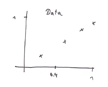
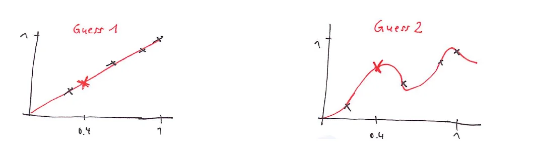
Both guesses on slide 41 fit the data perfectly. Which one is better cannot be decided from the data alone.

Consequence 1: inductive bias

We need to have an idea what we are looking for. This is called the “inductive bias”. Learning is impossible without such a bias.

Examples: $f$ is periodic (daily temperatures), $f$ is “simple” (caution, see learning theory later), similar inputs lead to similar outputs.

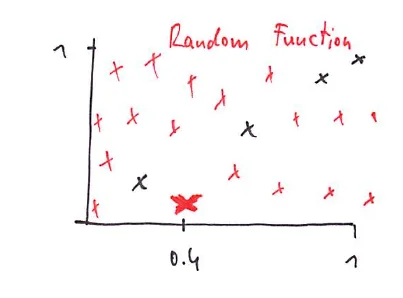
Now the lecturer reveals that the $Y_i$ were produced by a uniform random number generator (slide 43). Then no prediction for $0.4$ is better than any other.

Consequence 2: there must be a signal

We can only learn if there is something we can learn: the input has to contain some signal about the output (Y “has something to do” with X, there is a simple rule that produces the output).

Excursion: inductive bias in animal learning

Slides 45-47

Rats get two kinds of water, one makes them sick.

• Experiment 1: the two kinds taste differently. Rats learn very fast to avoid the water that makes them sick.
• Experiment 2: the same taste, but one kind comes with audio-visual stimuli (sounds, light). Rats do not learn to avoid it.

From the point of view of evolution, the taste of food is related to getting sick, sounds are not. The rat has an inductive bias. In psychology this is the Garcia effect (Garcia et al., 1960s).

Bottom line

Machine learning can only work on reasonable data. Any successful learning algorithm has an inherent inductive bias. For some algorithms the bias is obvious, for others it is hard to understand what it is and how to change it. But if the algorithm works, there has to be a bias. The rest of the course makes this precise.

Predicting based on perfect knowledge

The standard statistical setup

Slides 48-54

In this section we assume complete knowledge of the distribution and ask how to derive the best predictions from it (Bach Sec. 2, Devroye et al. Sec. 2, Hastie et al. Sec. 2.4-2.9).

Data spaces and distribution

• input space $\mathcal{X}$, output space $\mathcal{Y}$ (each with a $\sigma$-algebra, which we ignore)
• a probability distribution $P$ on $\mathcal{X}\times \mathcal{Y}$
• no assumption on the form of $P$, and both inputs and outputs are random quantities

Classifier, prediction function

A function $f:\mathcal{X}\to \mathcal{Y}$. If $\mathcal{Y}$ is discrete this is classification, if $\mathcal{Y}=\mathbb{R}$ it is regression (other outputs, for example structured prediction, are possible).

Loss function

A function $\ell :\mathcal{X}\times \mathcal{Y}\times \mathcal{Y}\to {\mathbb{R}}_{\ge 0}$ that measures how “expensive” an error is.

• 0-1 loss for classification: $\ell (x,y,y^{\prime })=0$ if $y=y^{\prime }$ and $1$ otherwise
• squared loss for regression: $\ell (x,y,y^{\prime })=(y-y^{\prime }{)}^2$

The choice of the loss influences the inductive bias.

Sometimes the loss has to depend on $x$ (a wrong medical decision is worse for some patients than for others), and sometimes on the order of $y$ and $y^{\prime }$: predicting “healthy” for a sick person is worse than the other way around. Later we often drop $x$ and write $\ell (y,y^{\prime })$.

True risk

Slide 55

True risk (true expected loss)

$$R(f):=E(\ell (X,Y,f(X)))$$

The expectation is over the random draw of $(X,Y)\sim P$. The goal of machine learning is to use the training data to construct a function $f_n$ whose true risk is as small as possible.

Bayes risk and Bayes classifier

Slide 56

Bayes risk and Bayes classifier

$$R^{\ast }:=\inf \{R(f)\mid f:\mathcal{X}\to \mathcal{Y}\text{ measurable}\}$$

If the infimum is attained, $f^{\ast }:={\mathrm{argmin}}_{f}R(f)$ is called the Bayes classifier (or Bayes predictor). It is not necessarily unique.

Trap

$R^{\ast }$ is a number (the smallest achievable risk), $f^{\ast }$ is a function. $R^{\ast }=0$ only if $Y$ is a deterministic function of $X$. With overlapping classes, even the Bayes classifier makes errors.

Optimal prediction functions in closed form

Classification under 0-1 loss: the regression function

Slides 57-62

Let $(X,Y)\sim P$ on $\mathcal{X}\times \{0,1\}$. We describe $P$ by two quantities:

Marginal and regression function

• $\mu$ is the marginal distribution of $X$: $\mu (A)=P(X\in A)$
• the regression function is $\eta (x):=E(Y\mid X=x)$. For binary classification,

$$\eta (x)=0\cdot P(Y=0\mid X=x)+1\cdot P(Y=1\mid X=x)=P(Y=1\mid X=x)$$

Intuition

If $\eta (x)$ is close to 0 or 1, classifying $x$ is easy: almost all points at $x$ have the same label. If $\eta (x)$ is close to $0.5$, both labels are about equally likely at $x$, and every classifier makes many errors there.

Proposition 1 (unique decomposition)

The distribution $P$ is uniquely determined by $\mu$ and $\eta$.

Intuition (discrete case):

$$P(X=x,Y=1)=\eta (x)\mu (x),P(X=x,Y=0)=(1-\eta (x))\mu (x)$$

The formal proof for the general case is in the first pages of Devroye, Györfi and Lugosi.

Mini example: from a joint table to $\mu$ and $\eta$

	$x=a$	$x=b$
$P(X=x,Y=1)$	0.10	0.45
$P(X=x,Y=0)$	0.30	0.15

$\mu (a)=0.40$, $\mu (b)=0.60$. $\eta (a)=0.10/0.40=0.25$, $\eta (b)=0.45/0.60=0.75$. Backwards: $\eta (b)\mu (b)=0.75\cdot 0.6=0.45$ gives the table again.

Explicit form of the Bayes classifier for the 0-1 loss

Slides 63-67

Under the 0-1 loss, the risk counts how often a classifier fails:

$$R(f)=E(\ell (X,Y,f(X)))=E(1_{f(X)\ne Y})=P(f(X)\ne Y)$$

The Bayes classifier $f^{\ast }$ was defined implicitly as the minimizer. Now consider

$$f^{\circ }(x):=\{\begin{array}{ll}1& \text{if }\eta (x)\ge 1/2\\ 0& \text{otherwise}\end{array}$$

Theorem 2 ( $f^{\circ }$ is a Bayes classifier)

Consider classification with the 0-1 loss. Let $f:\mathcal{X}\to \{0,1\}$ be any (measurable) classifier. Then

$$R(f)\ge R(f^{\circ })$$

So $f^{\circ }=f^{\ast }$: for the 0-1 loss we have an explicit formula for the Bayes classifier. In practice this does not help, because we do not know $\eta$.

Proof of Theorem 2

Step 1. Fix a classifier $f$ and a point $x$. Since $f(x)$ is deterministic (step $(\ast )$),

$$\begin{array}{rl}P(f(x)\ne Y\mid X=x)& =1-P(f(x)=Y\mid X=x)\\ & =1-P(f(x)=1,Y=1\mid X=x)-P(f(x)=0,Y=0\mid X=x)\\ & \stackrel{(\ast )}{=}1-1_{f(x)=1}\eta (x)-1_{f(x)=0}(1-\eta (x))\end{array}$$

Step 2. Compare the pointwise error of $f$ with the one of $f^{\circ }$. Plugging in step 1 and simplifying:

$$P(f(X)\ne Y\mid X=x)-P(f^{\circ }(X)\ne Y\mid X=x)=(2\eta (x)-1)(1_{f^{\circ }(x)=1}-1_{f(x)=1})\stackrel{(\ast \ast )}{\ge }0$$

For $(\ast \ast )$: if $f^{\circ }(x)=1$, then $\eta (x)\ge 0.5$ and both factors are $\ge 0$. If $f^{\circ }(x)=0$, then $\eta (x)\le 0.5$ and both factors are $\le 0$.

Step 3. The inequality $P(f(X)\ne Y\mid X=x)\ge P(f^{\circ }(X)\ne Y\mid X=x)$ holds for every $x$, so it also holds in expectation over $x$: $R(f)\ge R(f^{\circ })$. $\square$

Consequence: the Bayes error

Step 1 with $f=f^{\circ }$ gives the pointwise error $\min (\eta (x),1-\eta (x))$. So

$$\begin{array}{rl}{R}^{\ast }& =E[\min (\eta (X),1-\eta (X))]\\ & =\sum _x\min (P(X=x,Y=1),P(X=x,Y=0))\text{(discrete }X\text{)}\end{array}$$

In words: at every $x$, the Bayes classifier loses the smaller of the two joint probabilities.

Exam-style task: Bayes classifier on a discrete input (4 P)

Let $X\in \{0,1,2\}$ and $Y\in \{0,1\}$ with prior $P(Y=1)=0.3$ and class conditionals

$x$	0	1	2
$P(X=x\mid Y=1)$	0.1	0.3	0.6
$P(X=x\mid Y=0)$	0.5	0.3	0.2

(a) (1 P, easy) Compute $\mu (x)$ and $\eta (x)$ for all $x$ and state the 0-1 Bayes classifier.

(b) (1.5 P, harder) Compute the Bayes error. Then use the loss $\ell (y=1,\hat{y}=0)=a$, $\ell (y=0,\hat{y}=1)=1$ with $a=3$: which classifier is optimal now, and what is its risk?

(c) (1.5 P, backwards) For which values of $a$ does the optimal classifier predict 1 at $x=1$ (ties toward 1)?

Solution

(a) Joint probabilities $P(X=x,Y=1)=0.3\cdot P(X=x\mid Y=1)$: $0.03,0.09,0.18$. $P(X=x,Y=0)=0.7\cdot P(X=x\mid Y=0)$: $0.35,0.21,0.14$. So $\mu =(0.38,0.30,0.32)$ and $\eta =(0.03/0.38,0.09/0.30,0.18/0.32)\approx (0.079,0.30,0.5625)$. Bayes classifier: $f^{\ast }(0)=0$, $f^{\ast }(1)=0$, $f^{\ast }(2)=1$. (1 P)

(b) Bayes error $={\sum }_x\min ({\text{joint}}_1,{\text{joint}}_0)=0.03+0.09+0.14=0.26$ (0.5 P). With costs, predicting 0 at $x$ costs $a\eta (x)$ and predicting 1 costs $1-\eta (x)$, so predict 1 iff $\eta (x)>1/(1+a)=0.25$. Decisions: $(0,1,1)$, so $x=1$ flips. Risk: $3\cdot 0.03+0.21+0.14=0.44$ (the old rule would cost $0.09+0.27+0.14=0.50$). (1 P)

(c) Predict 1 at $x=1$ iff $\eta (1)=0.3\ge 1/(1+a)⟺1+a\ge 10/3⟺a\ge 7/3$. Missing a 1 must cost at least $7/3$ times as much as a false 1. (1.5 P)

→ Practice: Mock exam, task 3 (same structure, different numbers). Sheet 1, Exercise 3 for the $L_2$ version.

Other classification losses: scoring functions

Slides 68-73

The 0-1 loss is hard to work with: it is not continuous and not convex, so it cannot be optimized with gradients. So one uses other loss functions. To account for this, the setup changes slightly:

Scoring function

For binary classification with labels $\pm 1$, consider a real-valued scoring function $f:\mathcal{X}\to \mathbb{R}$ and threshold it at 0:

$$c_f(x)=\mathrm{sign}(f(x))$$

A point $(X,Y)$ is classified correctly iff $f(X)\cdot Y>0$. The product $Yf(X)$ is the margin.

The Bayes predictor is the scoring function that minimizes the risk, $f^{\ast }={\mathrm{argmin}}_{f}R(f)$, and the classifier is $c^{\ast }(x)=\mathrm{sign}(f^{\ast }(x))$. With labels $\pm 1$ the regression function becomes

$${\eta }_1(x):=E(Y\mid X=x)=P(Y=1\mid X=x)-P(Y=-1\mid X=x)\in [-1,1]$$

so $\eta (x)=(1+{\eta }_1(x))/2$ and $1-\eta (x)=(1-{\eta }_1(x))/2$. The 0-1 Bayes classifier is $+1$ iff $\eta (x)>0.5$ iff ${\eta }_1(x)>0$.

There are many losses in this regime: hinge, squared, exponential, logistic. For binary classification, the cross-entropy loss coincides with the logistic loss.

Slide 73: losses as functions of the margin y·f(x). Negative margin: wrongly classified, positive margin: correctly classified.

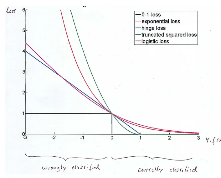
Bayes predictors for various loss functions

Slides 74-78

Bayes predictors (slide 74)

name	loss $\ell (y,f(x))$	Bayes predictor $f^{\ast }$	classifier $c_{f^{\ast }}$
hinge	$\max (0,1-yf(x))$	$+1$ if ${\eta }_1(x)>0$, $-1$ if ${\eta }_1(x)<0$	$+1$ iff ${\eta }_1(x)>0$
squared	$\max (0,1-yf(x){)}^2$	${\eta }_1(x)$	$+1$ iff ${\eta }_1(x)>0$
exponential	$\exp (-yf(x))$	$\frac{1}{2}\log \frac{1+{\eta }_1(x)}{1-{\eta }_1(x)}$	$+1$ iff ${\eta }_1(x)>0$
logistic	${\log }_2(1+\exp (-yf(x)))$	$\log \frac{1+{\eta }_1(x)}{1-{\eta }_1(x)}$	$+1$ iff ${\eta }_1(x)>0$

Two observations (slide 75)

• Different losses give different Bayes predictors: they induce different inductive biases, because they prefer slightly different scoring functions.
• Surprisingly, the thresholded classifiers are all the same and coincide with the Bayes classifier under the 0-1 loss. This property has a name: the loss is classification-calibrated (more later in the course).

Proof for the exponential loss

Risk at a point $x$. The scores are real, the labels are still $\pm 1$:

$$\begin{array}{rl}{R}_x(f)& =P(Y=1\mid X=x)\ell (f(x),1)+P(Y=-1\mid X=x)\ell (f(x),-1)\\ & =\frac{1+{\eta }_1(x)}{2}{e}^{-f(x)}+\frac{1-{\eta }_1(x)}{2}{e}^{f(x)}\end{array}$$

Minimum. Write $t:=f(x)$ and set the derivative to zero (${\eta }_1(x)$ is a constant here):

$$\frac{\partial R_x(t)}{\partial t}=-\frac{1+{\eta }_1(x)}{2}{e}^{-t}+\frac{1-{\eta }_1(x)}{2}{e}^t\stackrel{!}{=}0\Rightarrow t^{\ast }=f^{\ast }(x)=\frac{1}{2}\log \frac{1+{\eta }_1(x)}{1-{\eta }_1(x)}$$

The second derivative at $t^{\ast }$ is $>0$, and the function is convex, so this is the global minimum.

Classifier. $f^{\ast }(x)>0⟺\frac{1+{\eta }_1}{1-{\eta }_1}>1⟺{\eta }_1(x)>0$. $\square$

Mini example: $\eta (x)=0.8$

Then ${\eta }_1(x)=2\cdot 0.8-1=0.6$ and $\frac{1+{\eta }_1}{1-{\eta }_1}=\frac{1.6}{0.4}=4$.

• hinge: $f^{\ast }(x)=+1$
• squared: $f^{\ast }(x)=0.6$
• exponential: $f^{\ast }(x)=\frac{1}{2}\ln 4\approx 0.69$
• logistic: $f^{\ast }(x)=\ln 4\approx 1.39$

Four different scores, one label: all are positive, so all predict $+1$, like the 0-1 Bayes classifier ($\eta =0.8>0.5$).

Left: the losses as functions of the margin. Right: the conditional risk at a point with the chosen η(x), with the minimizer of each loss marked. Move η across 0.5 and watch all minimizers change sign together.

The exponential loss comes back in Lecture 6: AdaBoost minimizes it.

Regression under the squared loss

Slides 79-84

Regression looks similar, with one important difference: $Y$ can be any real number, so we cannot split into the two cases $Y=\pm 1$. Conditional expectations are integrals, not sums. Consider the squared loss $\ell (x,y,f(x))=(f(x)-y{)}^2$ and the regression function $\eta (x)=E(Y\mid X=x)$.

Proposition 3 (decomposition)

$$E(|f(X)-Y{|}^2)=E(|f(X)-\eta (X){|}^2)+E(|\eta (X)-Y{|}^2)$$

An inequality with $\le$ would be trivial (triangle inequality). The equality is not.

Proof of Proposition 3

Add and subtract $\eta (X)$ and expand the square:

$$E|f(X)-Y{|}^2=E((f(X)-\eta (X){)}^2)+E((\eta (X)-Y{)}^2)+2\underset{(\#)}{\underbrace{E((f(X)-\eta (X))(\eta (X)-Y))}}$$

The mixed term $(\#)$ is 0. By the tower property $E(Z)=E(E(Z\mid X))$, and because $f(X)-\eta (X)$ is a function of $X$ it can be pulled out of the inner conditional expectation:

$$(\#)=E\left(\right(f(X)-\eta (X)\left)E\right(\eta (X)-Y\mid X\left)\right)=E\left(\right(f(X)-\eta (X)\left)\right(\eta (X)-E(Y\mid X)\left)\right)=0$$

since $E(Y\mid X)=\eta (X)$. (Details with conditional expectations: Györfi, Kohler, Krzyżak and Walk, p. 2.) $\square$

Theorem 4 (explicit form of the optimal $L_2$ solution)

The function $f^{\circ }(x):=\eta (x)=E(Y\mid X=x)$ minimizes the $L_2$ risk.

Proof: in Proposition 3, the second term does not depend on $f$. The first term is $\ge 0$ and equals 0 for $f(X)=\eta (X)$. $\square$

Mini example: Bayes predictor and Bayes risk for the squared loss

$X\in \{0,1\}$ with $P(X=0)=P(X=1)=0.5$. Given $X=0$, $Y$ is 1 or 3 with probability $1/2$ each. Given $X=1$, $Y$ is 2 or 6.

• $\eta (0)=2$, $\eta (1)=4$: this is $f^{\ast }$.
• Bayes risk $=E|\eta (X)-Y{|}^2=E[\mathrm{Var}(Y\mid X)]=0.5\cdot 1+0.5\cdot 4=2.5$.
• The constant $f\equiv 3$ has risk $E|f-\eta {|}^2+2.5=0.5\cdot 1+0.5\cdot 1+2.5=3.5$.

The same result in Sheet 1, Exercise 3: minimize $r(q)=E((Y-q{)}^2\mid X=x)$ pointwise, $r^{\prime }(q)=-2E(Y\mid X=x)+2q=0$ gives $q^{\ast }=E(Y\mid X=x)$, and the Bayes risk is $E[\mathrm{Var}(Y\mid X)]$: the noise that no predictor can remove.

Statistical and Bayesian decision theory

More than just Bayes classifiers

Slides 85-88

So far we derived the explicit Bayes classifier for particular losses. Now we look at several ways to come up with “perfect classifiers” in a slightly more abstract setting (Hastie Sec. 2.4-2.9, Devroye Sec. 2).

Running example: predict the gender of a person from the body height. We know the class conditional distributions $P(X\mid Y)$ (two bell curves, the female one peaks around 165 cm, the male one around 178 cm). How would you label $X=160$?

Approach 1: just look at the priors

Slides 89-90

Decide based on the class priors $P(Y)$ only: always predict the label of the larger class.

$$f_n(X)=\{\begin{array}{ll}m& \text{if }P(Y=m)>P(Y=f)\\ f& \text{otherwise}\end{array}$$

Visually: select the higher bar. This ignores $X$ completely (“a bit stupid”). Its error is $\min ({\pi }_0,{\pi }_1)$.

Approach 2: maximum likelihood principle

Slides 91-92

Decide based on the likelihood functions $P(X\mid Y)$, the class conditional distributions $P(X\mid Y=m)$ and $P(X\mid Y=f)$. Predict the label with the higher likelihood:

$$f_n(x)=\{\begin{array}{ll}m& \text{if }P(X=x\mid Y=m)>P(X=x\mid Y=f)\\ f& \text{otherwise}\end{array}$$

Visually: select according to which class-conditional curve is higher. ML ignores the priors.

Approach 3: Bayesian a posteriori criterion

Slides 93-94

Decide based on the posterior distributions $P(Y\mid X)$ (Bayesian maximum a posteriori, MAP). Compute

$$P(Y=m\mid X=x)=\frac{P(X=x\mid Y=m)\cdot P(Y=m)}{P(X=x)}$$

and predict $m$ iff $P(Y=m\mid X=x)>P(Y=f\mid X=x)$. Visually: select according to which posterior curve is higher. The denominator $P(X=x)$ is the same for both classes, so MAP compares $P(X=x\mid Y=y)P(Y=y)$.

MAP = Bayes classifier for the 0-1 loss

The MAP rule is exactly $f^{\circ }$ from Theorem 2: predict 1 iff $\eta (x)\ge 1/2$. With a uniform prior, MAP and ML coincide.

Approach 4: take the costs of errors into account

Slide 95

Bayes decision rule

• A loss $\ell (x,y,\hat{y})$ says how much we lose by predicting $\hat{y}$ when the true label is $y$.
• The conditional risk at $x$ is the expected loss when predicting $\hat{y}$ (randomness only in the true label $Y$ of $x$):

$$\begin{array}{rl}R(\hat{y}\mid X=x)=& \ell (x,m,\hat{y})P(Y=m\mid X=x)\\ +& \ell (x,f,\hat{y})P(Y=f\mid X=x)\end{array}$$

• Bayes decision rule: select the label $f_n(x)$ for which the conditional risk is minimal.

For two classes $\{0,1\}$ write ${\ell }_{\hat{y}y}$ for the loss of predicting $\hat{y}$ when the truth is $y$ (correct predictions cost 0). Then ${\ell }_{01}$ is the cost of missing a 1 and ${\ell }_{10}$ the cost of a false 1:

$$R(1\mid x)={\ell }_{10}(1-\eta (x)),R(0\mid x)={\ell }_{01}\eta (x)$$

Two-class Bayes decision rule (the one formula for the exam)

Predict 1 iff $R(1\mid x)<R(0\mid x)$, equivalently

$$\begin{array}{rl}& \eta (x)>\frac{{\ell }_{10}}{{\ell }_{10}+{\ell }_{01}}\\ ⟺& {\pi }_1{\ell }_{01}p(x\mid 1)>{\pi }_0{\ell }_{10}p(x\mid 0)\\ ⟺& \frac{p(x\mid 1)}{p(x\mid 0)}>\frac{{\pi }_0{\ell }_{10}}{{\pi }_1{\ell }_{01}}\end{array}$$

• 0-1 loss (${\ell }_{01}={\ell }_{10}$): MAP, threshold $\eta >1/2$.
• additionally uniform prior: ML, likelihood ratio $>1$.
• The decision boundaries are the points where ${\pi }_1{\ell }_{01}p(x\mid 1)={\pi }_0{\ell }_{10}p(x\mid 0)$: where the two weighted curves cross.

With the mock exam’s notation $\ell (y=1,\hat{y}=0)=a$, $\ell (y=0,\hat{y}=1)=1$ this is $\eta (x)>1/(1+a)$.

flowchart LR
  A["priors P(Y)"] --> R1["Approach 1: larger class"]
  B["likelihoods P(X|Y)"] --> R2["Approach 2: maximum likelihood"]
  A & B --> C["posterior P(Y|X) (Bayes rule)"] --> R3["Approach 3: MAP = Bayes classifier for 0-1 loss"]
  C & D["costs ℓ"] --> R4["Approach 4: Bayes decision rule, minimal conditional risk"]

Which way does the boundary move?

Increasing ${\pi }_1$ or ${\ell }_{01}$ makes class 1 “cheaper to predict”: the region where we predict 1 grows, and the boundary moves towards class 0. On the slides: with prior $P(\text{male})=0.8$ the threshold moves from about 172 cm to about 160 cm, and people are called male at smaller heights.

Simulations: the lecturer’s demo

Slides 96-104

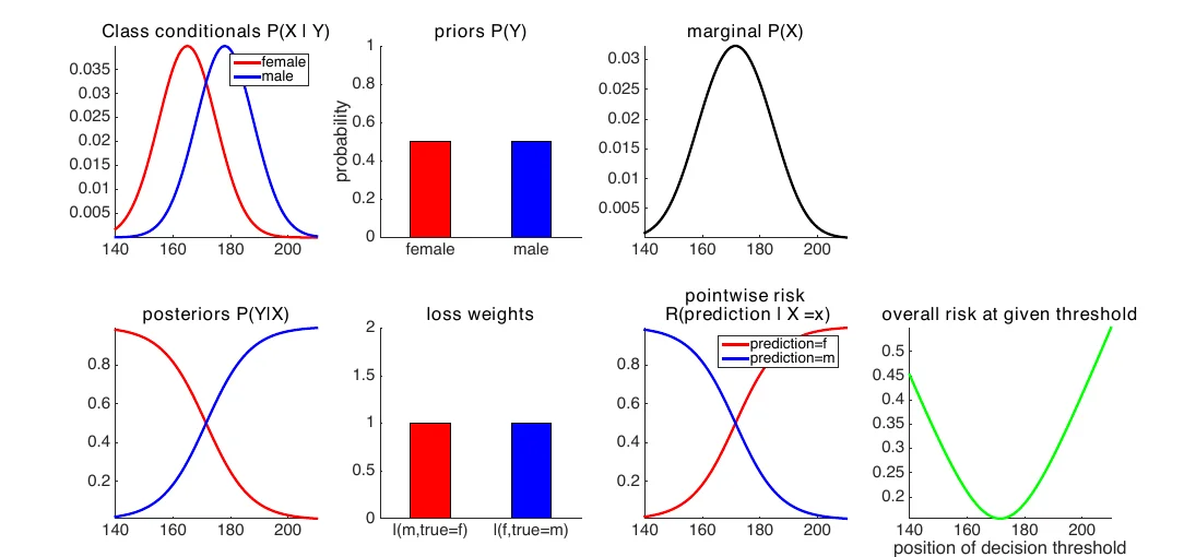
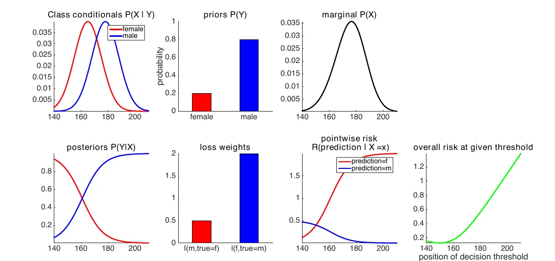
The slides show simulations (script demo_bayesian_decision_theory.py) for the stylized model $X\in \mathbb{R}$ height, $Y\in \{m,f\}$ gender. Each panel shows: class conditionals $P(X\mid Y)$, priors $P(Y)$, marginal $P(X)=P(X\mid Y=f){\pi }_f+P(X\mid Y=m){\pi }_m$, posteriors $P(Y\mid X)$, the loss weights, the pointwise risk $R(\text{prediction}\mid X=x)$ and the overall risk of a threshold $t$ (everybody with height $\le t$ is predicted female).

Slide 97: equal priors, equal losses. The optimal threshold sits where the posteriors cross.

Slide 100: P(m) = 0.8 and calling a male "female" costs 2 (the other error 0.5). The threshold moves far to the left.

Slide	Priors $({\pi }_f,{\pi }_m)$	Losses $\ell (m,\text{true }f)$, $\ell (f,\text{true }m)$	Optimal threshold
97	0.5, 0.5	1, 1	in the middle (≈ 172 cm)
98	0.2, 0.8	1, 1	lower (≈ 160 cm): more people are called male
99	0.5, 0.5	0.5, 2	lower: missing a male is expensive
100	0.2, 0.8	0.5, 2	much lower: both effects push the same way
101	0.2, 0.8	2, 0.5	back up (≈ 172 cm): prior and costs cancel

On slide 101 the effects cancel exactly: ${\pi }_f\ell (m,\text{true }f)=0.2\cdot 2=0.4=0.8\cdot 0.5={\pi }_m\ell (f,\text{true }m)$, so the weighted curves are the unweighted ones scaled by the same factor.

Risk of a threshold rule (slides 102-104)

With “predict $f$ iff $x\le t$”, all males below $t$ and all females above $t$ are misclassified:

$$\begin{array}{rl}{R}_t& ={\ell }_{fm}P(Y=m,X\le t)+{\ell }_{mf}P(Y=f,X>t)\\ & ={\ell }_{fm}{\int }_{-\infty }^{t}P(Y=m\mid X=x)p(x)dx\\ & +{\ell }_{mf}{\int }_t^{\infty }P(Y=f\mid X=x)p(x)dx\end{array}$$

where ${\ell }_{fm}$ is the loss for predicting $f$ when the truth is $m$, and $p(x)$ the marginal density.

Trap

The slides write this in short form as $P(Y=m\mid X\in ]-\infty ,t])$ and $\int P(Y=m\mid X=x)dx$. Written out exactly, the probabilities are joint probabilities, and inside the integral the posterior is weighted with the marginal density $p(x)$. Equivalently, $P(Y=m,X\le t)={\pi }_m{\int }_{-\infty }^{t}p(x\mid m)dx$.

The demo of slides 96-104 to play with. Change priors and costs and watch the Bayes, ML and MAP boundaries, the posterior with its threshold and the risk of every threshold. The exam presets use boxes and triangles like in the tasks below.

Reading decision boundaries off a diagram

This section is exam training for the real exam’s Bayes task: you get a diagram of the class-conditional densities (often boxes or triangles, sometimes Gaussians) and have to determine the decision rule mathematically.

Recipe

1. Read the densities $p(x\mid 0)$ and $p(x\mid 1)$ off the diagram and write them as formulas on each piece where they are non-zero.
2. Weight them: $g_0(x)={\pi }_0{\ell }_{10}p(x\mid 0)$ and $g_1(x)={\pi }_1{\ell }_{01}p(x\mid 1)$. (ML: no weights. MAP: priors only.)
3. Where only one class has density, predict that class. In the overlap, predict 1 where $g_1>g_0$.
4. Boundary: solve $g_1(x)=g_0(x)$ on the overlap (constant pieces: compare heights; linear pieces: a linear equation; Gaussians with equal variance: a linear equation in $x$ after taking logs).
5. Error of the rule: integrate the smaller weighted curve, $R^{\ast }=\int \min (g_0,g_1)dx$ (with $\pi$ only, without costs, for the 0-1 error).
6. Backwards: plug the given boundary $x_b$ into $g_1(x_b)=g_0(x_b)$ and solve for the unknown prior or cost ratio.

Exam-style task: boxes (4 P)

(a) (1 P, easy) Give the maximum likelihood decision rule.

(b) (1.5 P, harder) Let $P(Y=1)=0.7$ and use the 0-1 loss. Give the Bayes classifier and its error.

(c) (1.5 P, backwards) For which priors ${\pi }_1$ does the 0-1 Bayes classifier predict 1 on $[2,4]$? With a uniform prior instead, which cost ratio ${\ell }_{01}/{\ell }_{10}$ achieves the same?

Solution

(a) On $[0,2)$ only class 0 has density: predict 0. On $[2,4]$: $p(x\mid 0)=1/4>1/6=p(x\mid 1)$: predict 0. On $(4,8]$ only class 1: predict 1. So $f_{ML}(x)=1$ iff $x>4$. (1 P)

(b) On $[2,4]$: ${\pi }_{0}p(x\mid 0)=0.3\cdot 1/4=0.075<{\pi }_{1}p(x\mid 1)=0.7\cdot 1/6\approx 0.117$: predict 1. So $f^{\ast }(x)=1$ iff $x\ge 2$ (1 P). Error: only on the overlap, where the smaller weighted curve is $0.075$: $R^{\ast }=2\cdot 0.075=0.15$. (0.5 P)

(c) Predict 1 on $[2,4]$ iff ${\pi }_1/6>(1-{\pi }_1)/4⟺4{\pi }_1>6-6{\pi }_1⟺{\pi }_1>0.6$ (at ${\pi }_1=0.6$ both labels are optimal on $[2,4]$). (1 P) Uniform prior: iff ${\ell }_{01}/6>{\ell }_{10}/4⟺{\ell }_{01}/{\ell }_{10}>1.5$. (0.5 P)

Exam-style task: triangles (4 P)

(a) (1 P, easy) Write down both densities on the overlap $[2,4]$ and give the ML boundary.

(b) (1.5 P, harder) Let $P(Y=1)=1/3$ with the 0-1 loss. Compute the Bayes boundary and the Bayes error.

(c) (1.5 P, backwards) The 0-1 Bayes classifier has its boundary at $x=2.5$. Which prior ${\pi }_1$ was used?

Solution

(a) On $[2,4]$ the red triangle falls from $1/2$ to 0 and the blue one rises from 0 to $1/2$: $p(x\mid 0)=(4-x)/4$, $p(x\mid 1)=(x-2)/4$. ML boundary: $4-x=x-2\Rightarrow x=3$. (1 P)

(b) $\frac{2}{3}\cdot \frac{4-x}{4}=\frac{1}{3}\cdot \frac{x-2}{4}\Rightarrow 8-2x=x-2\Rightarrow x^{\ast }=10/3\approx 3.33$ (0.75 P). Error: class-1 mass left of $x^{\ast }$ plus class-0 mass right of $x^{\ast }$: $\frac{1}{3}{\int }_2^{10/3}\frac{x-2}{4}dx+\frac{2}{3}{\int }_{10/3}^4\frac{4-x}{4}dx=\frac{1}{3}\cdot \frac{(4/3{)}^2}{8}+\frac{2}{3}\cdot \frac{(2/3{)}^2}{8}=\frac{2}{27}+\frac{1}{27}=\frac{1}{9}\approx 0.111$. (0.75 P)

(c) At $x=2.5$: ${\pi }_0\cdot (4-2.5)={\pi }_1\cdot (2.5-2)\Rightarrow 1.5{\pi }_0=0.5{\pi }_1\Rightarrow {\pi }_1=3{\pi }_0\Rightarrow {\pi }_1=0.75$. The boundary moved towards class 0, so class 1 must be more likely. (1.5 P)

Exam-style task: Gaussians with equal variance (4 P)

$p(x\mid y)=\mathcal{N}({\mu }_y,{\sigma }^2)$ with ${\mu }_0=2$, ${\mu }_1=6$, $\sigma =2$.

(a) (1 P, easy) Give the boundary for the uniform prior and the 0-1 loss.

(b) (1.5 P, harder) Show that in general the boundary is $x^{\ast }=\frac{{\mu }_0+{\mu }_1}{2}+\frac{{\sigma }^2}{{\mu }_1-{\mu }_0}\ln \frac{{\pi }_0{\ell }_{10}}{{\pi }_1{\ell }_{01}}$ and evaluate it for ${\pi }_1=0.25$ with the 0-1 loss.

(c) (1.5 P, backwards) With a uniform prior the observed boundary is $x^{\ast }=3$. What cost ratio ${\ell }_{01}/{\ell }_{10}$ was used? Interpret.

Solution

(a) By symmetry, where the two bell curves cross: $x^{\ast }=(2+6)/2=4$. (1 P)

(b) Predict 1 iff $\ln ({\pi }_1{\ell }_{01}p(x\mid 1))>\ln ({\pi }_0{\ell }_{10}p(x\mid 0))$. The normalizing constants cancel, and $(x-{\mu }_0{)}^2-(x-{\mu }_1{)}^2=({\mu }_1-{\mu }_0)(2x-{\mu }_0-{\mu }_1)$, so the condition is $\frac{({\mu }_1-{\mu }_0)(2x-{\mu }_0-{\mu }_1)}{2{\sigma }^2}>\ln \frac{{\pi }_0{\ell }_{10}}{{\pi }_1{\ell }_{01}}$, which for ${\mu }_1>{\mu }_0$ gives $x>x^{\ast }$ with the formula above (1 P). For ${\pi }_1=0.25$: $x^{\ast }=4+\frac{4}{4}\ln 3\approx 5.10$. (0.5 P)

(c) $3=4+1\cdot \ln ({\ell }_{10}/{\ell }_{01})\Rightarrow {\ell }_{01}/{\ell }_{10}=e\approx 2.72$. Missing a 1 costs about 2.7 times as much as a false 1, so the rule predicts 1 already from $x=3$ on. (1.5 P)

Unequal variances

If ${\sigma }_0\ne {\sigma }_1$, the log-likelihood ratio is quadratic in $x$ and there can be two boundaries: the class with the wider density wins on both sides. Then no single threshold is optimal. Try the preset “Unequal spreads” in the explorer above.

Exam-style task: three classes (4 P)

Three classes with box densities: $p(x\mid A)=1/2$ on $[0,2]$, $p(x\mid B)=1/4$ on $[1,5]$, $p(x\mid C)=1/3$ on $[4,7]$.

(a) (1 P) Give the ML rule on $[0,7]$.

(b) (1.5 P) Priors ${\pi }_A=0.2$, ${\pi }_B=0.5$, ${\pi }_C=0.3$, 0-1 loss. Give the MAP rule.

(c) (1.5 P) With the uniform prior, give a loss that makes the Bayes rule never predict $B$.

Solution

(a) $[0,1)$: only A. $[1,2]$: $1/2>1/4$, A. $(2,4)$: only B. $[4,5]$: $1/3>1/4$, C. $(5,7]$: only C. So A on $[0,2]$, B on $(2,4)$, C on $[4,7]$. (1 P)

(b) Weighted heights: A $0.2\cdot 0.5=0.1$, B $0.5\cdot 0.25=0.125$, C $0.3\cdot 1/3=0.1$. On $[1,2]$: B beats A. On $[4,5]$: B beats C. So A on $[0,1)$, B on $[1,5]$, C on $(5,7]$. (1.5 P)

(c) Make predicting $B$ very expensive: loss $C$ for predicting $B$ when the truth is A or C (large $C$, also $C=\infty$), 1 for all other errors. The conditional risk of predicting B is $C(1-P(B\mid x))$, which is larger than the risk of A or C (at most 1) wherever another class has density. This is the idea of Sheet 1, Exercise 2(c). (1.5 P)

Summary

Approach	Uses	Rule (two classes)	Boundary where
1. Priors only	$P(Y)$	larger class, always	no boundary
2. Maximum likelihood	$P(X\mid Y)$	$p(x\mid 1)>p(x\mid 0)$	class conditionals cross
3. MAP (= 0-1 Bayes classifier)	$P(X\mid Y)$, $P(Y)$	$\eta (x)>1/2$	${\pi }_{1}p(x\mid 1)={\pi }_{0}p(x\mid 0)$
4. Bayes decision rule	posterior and costs	$\eta (x)>{\ell }_{10}/({\ell }_{10}+{\ell }_{01})$	${\pi }_1{\ell }_{01}p(x\mid 1)={\pi }_0{\ell }_{10}p(x\mid 0)$

Loss	Bayes predictor	Bayes risk
0-1	$1_{\eta (x)\ge 1/2}$	$E[\min (\eta (X),1-\eta (X))]$
squared (regression)	$\eta (x)=E(Y\mid X=x)$	$E[\mathrm{Var}(Y\mid X)]$
hinge, squared, exponential, logistic (scores)	see the table above	thresholded: same classifier as 0-1

Self-Test

Question cards (14)

What is the difference between deductive and inductive inference, and what does it have to do with machine learning?

Answer

Deduction goes from general premises to certain conclusions; induction generalizes from specific examples, and the conclusion can be wrong. Machine learning tries to automate inductive inference.

What is an inductive bias, and why can no learning algorithm work without one?

Answer

An idea of what we are looking for, for example that $f$ is periodic, simple, or that similar inputs have similar outputs. Finitely many data points are fit by infinitely many functions (slide 41), so without a preference among them nothing can be predicted at a new point.

Besides an inductive bias, what else is needed for learning?

Answer

A signal: the input must contain information about the output. If $Y$ is produced by a random number generator independent of $X$, no prediction at $0.4$ is better than any other.

Define the true risk, the Bayes risk and the Bayes classifier.

Answer

$R(f)=E(\ell (X,Y,f(X)))$ with $(X,Y)\sim P$. $R^{\ast }={\inf }_{f}R(f)$ over all measurable $f$. If the infimum is attained, a minimizer $f^{\ast }=\mathrm{argmin}R(f)$ is a Bayes classifier; it need not be unique.

What is the regression function in binary classification, and what does it say about how hard a point is?

Answer

$\eta (x)=E(Y\mid X=x)=P(Y=1\mid X=x)$. Near 0 or 1 the label is almost determined (easy), near 0.5 both labels are equally likely (hard). Together with the marginal $\mu$ it determines $P$ uniquely (Proposition 1).

State Theorem 2 and explain why it does not help in practice.

Answer

For the 0-1 loss, $f^{\circ }(x)=1_{\eta (x)\ge 1/2}$ satisfies $R(f)\ge R(f^{\circ })$ for every classifier $f$, so it is a Bayes classifier. In practice $\eta$ is unknown; we only have a sample.

Sketch the proof of Theorem 2.

Answer

Pointwise error of any $f$: $1-1_{f(x)=1}\eta (x)-1_{f(x)=0}(1-\eta (x))$. The difference to $f^{\circ }$ is $(2\eta (x)-1)(1_{f^{\circ }(x)=1}-1_{f(x)=1})\ge 0$, because both factors have the same sign. Taking the expectation over $x$ gives $R(f)\ge R(f^{\circ })$.

What is the Bayes error for the 0-1 loss as a formula?

Answer

$R^{\ast }=E[\min (\eta (X),1-\eta (X))]$; for discrete $X$, ${\sum }_x\min (P(X=x,Y=1),P(X=x,Y=0))$.

Why use surrogate losses and scoring functions instead of the 0-1 loss, and what does "classification-calibrated" mean?

Answer

The 0-1 loss is not continuous and not convex, so it is hard to optimize. Surrogate losses on real scores (hinge, squared, exponential, logistic) are convex. Classification-calibrated: the sign of the loss’s Bayes predictor equals the 0-1 Bayes classifier, even though the scores themselves differ.

Derive the Bayes predictor for the exponential loss.

Answer

$R_x(t)=\frac{1+{\eta }_1}{2}{e}^{-t}+\frac{1-{\eta }_1}{2}{e}^t$. Setting the derivative to 0 gives $e^{2t}=\frac{1+{\eta }_1}{1-{\eta }_1}$, so $f^{\ast }(x)=\frac{1}{2}\log \frac{1+{\eta }_1(x)}{1-{\eta }_1(x)}$; the function is convex, so it is the global minimum, and $f^{\ast }>0$ iff ${\eta }_1>0$.

What is the Bayes predictor for regression with the squared loss, and why?

Answer

$f^{\ast }(x)=\eta (x)=E(Y\mid X=x)$. By Proposition 3, $E|f(X)-Y{|}^2=E|f(X)-\eta (X){|}^2+E|\eta (X)-Y{|}^2$; the second term does not depend on $f$, the first is 0 for $f=\eta$. The Bayes risk is $E[\mathrm{Var}(Y\mid X)]$.

Name the four approaches of decision theory and when two of them coincide.

Answer

Priors only, maximum likelihood, maximum a posteriori, and the Bayes decision rule with costs. MAP = ML for a uniform prior; the Bayes decision rule = MAP for the 0-1 loss.

Derive the two-class Bayes decision rule with costs ${\ell }_{01}$ (miss a 1) and ${\ell }_{10}$ (false 1).

Answer

$R(1\mid x)={\ell }_{10}(1-\eta (x))$ and $R(0\mid x)={\ell }_{01}\eta (x)$. Predict 1 iff ${\ell }_{10}(1-\eta )<{\ell }_{01}\eta$, i.e. $\eta (x)>{\ell }_{10}/({\ell }_{10}+{\ell }_{01})$, equivalently ${\pi }_1{\ell }_{01}p(x\mid 1)>{\pi }_0{\ell }_{10}p(x\mid 0)$.

How do you get a prior from a given decision boundary $x_b$ (0-1 loss)?

Answer

At the boundary the weighted densities are equal: ${\pi }_{1}p(x_b\mid 1)=(1-{\pi }_1)p(x_b\mid 0)$. Solve for ${\pi }_1=p(x_b\mid 0)/(p(x_b\mid 0)+p(x_b\mid 1))$. With costs and a uniform prior, solve ${\ell }_{01}p(x_b\mid 1)={\ell }_{10}p(x_b\mid 0)$ for the cost ratio instead.

Multiple Choice

Multiple choice (7)

Under the 0-1 loss, which classifier is a Bayes classifier?

• $f(x)=1$ iff $P(X=x\mid Y=1)\ge P(X=x\mid Y=0)$

• $f(x)=1$ iff $P(Y=1\mid X=x)\ge 1/2$

• $f(x)=1$ iff $P(Y=1)\ge 1/2$

• $f(x)=1$ iff $\eta (x)\ge \mu (x)$

Explanation

Theorem 2: threshold the posterior $\eta (x)$ at $1/2$. The first option is the ML rule; it ignores the prior and is only optimal for a uniform prior. The third ignores $x$ (approach 1). The fourth compares two unrelated quantities.

Let ${\ell }_{01}=4$ be the cost of predicting 0 when $Y=1$ and ${\ell }_{10}=1$ the cost of predicting 1 when $Y=0$. The Bayes decision rule predicts 1 iff

• $\eta (x)>0.8$

• $\eta (x)>0.5$

• $\eta (x)>0.2$

• $\eta (x)>0.25$

Explanation

The threshold is ${\ell }_{10}/({\ell }_{10}+{\ell }_{01})=1/5$. Missing a 1 is expensive, so we predict 1 already at small posteriors. $0.8$ swaps the roles of the costs, $0.25=1/4$ forgets to add ${\ell }_{10}$ in the denominator.

When do the maximum likelihood rule and the MAP rule always coincide?

• when the class conditionals are Gaussian

• when the prior is uniform

• when the loss is the 0-1 loss

• when both class conditionals have the same variance

Explanation

MAP compares $p(x\mid y){\pi }_y$, ML compares $p(x\mid y)$. They agree for all densities iff all ${\pi }_y$ are equal. The 0-1 loss is what makes MAP the Bayes classifier, not what makes it equal to ML. Equal variances only make the boundary a single point; a non-uniform prior still shifts it.

Which statement about the squared loss in regression is true?

• The Bayes predictor is the conditional median of $Y$ given $X=x$.

• The Bayes risk equals $E[\mathrm{Var}(Y\mid X)]$.

• The Bayes risk is 0 if $\eta$ is linear.

• $E|f(X)-Y{|}^2\le E|f(X)-\eta (X){|}^2+E|\eta (X)-Y{|}^2$ holds with strict inequality in general.

Explanation

Theorem 4: the Bayes predictor is the conditional mean $\eta (x)$ (the median belongs to the absolute loss), and the remaining risk is the conditional variance. The risk is 0 only without noise, independent of the shape of $\eta$. Proposition 3 is an equality.

The hinge, squared, exponential and logistic losses are classification-calibrated. This means:

• they all have the same Bayes predictor $f^{\ast }$

• $\mathrm{sign}(f^{\ast })$ is the 0-1 Bayes classifier for each of them

• each of them has the Bayes predictor $f^{\ast }(x)={\eta }_1(x)$

• their Bayes risk equals the 0-1 Bayes risk

Explanation

The Bayes predictors differ (${\eta }_1$ only for the squared loss, $\frac{1}{2}\log \frac{1+{\eta }_1}{1-{\eta }_1}$ for the exponential loss, …), but after thresholding at 0 they all give $+1$ iff ${\eta }_1>0$. The risks are measured in different losses, so their Bayes risks are different numbers.

Two classes, 0-1 loss. You increase the prior ${\pi }_1$ of class 1. What happens to the MAP decision region of class 1?

• it grows, the boundary moves towards class 0

• it shrinks, the boundary moves towards class 1

• it stays the same, because the likelihoods did not change

• it grows only if the class conditionals are Gaussian

Explanation

Class 1 wins where ${\pi }_{1}p(x\mid 1)>{\pi }_{0}p(x\mid 0)$. A larger ${\pi }_1$ scales up the left side everywhere, so the region grows for any shape of densities. Only ML ignores the prior.

Box densities: $p(x\mid 0)=1/2$ on $[0,2]$, $p(x\mid 1)=1/4$ on $[1,5]$, 0-1 loss. For which prior does the Bayes classifier predict 1 on $[1,2]$?

• ${\pi }_1>1/2$

• ${\pi }_1>2/3$

• ${\pi }_1>1/3$

• never, because $p(x\mid 0)>p(x\mid 1)$ there

Explanation

${\pi }_1/4>(1-{\pi }_1)/2⟺{\pi }_1>2(1-{\pi }_1)⟺{\pi }_1>2/3$. The last option is the ML answer, which ignores the prior.

References

All sources cited on the slides, in slide order (16 entries)

Slide	Source	Key point
6	Hardt and Recht, Patterns, Predictions, and Actions, 2022, introduction (online)	history of AI and ML
11	Minsky and Papert, Perceptrons, 1969	single-layer perceptrons cannot learn XOR
12	Lighthill, Artificial Intelligence: A General Survey (Lighthill Report), 1973	AI winter
22	Vaswani et al., “Attention Is All You Need”, NeurIPS 2017	transformers
32	Hardt and Recht, Patterns, Predictions, and Actions, 2022 (online)	main textbook
32	Shalev-Shwartz and Ben-David, Understanding Machine Learning, 2014 (online)	main textbook
32	Bach, Learning Theory from First Principles, 2024	additional textbook
32	Hastie, Tibshirani and Friedman, The Elements of Statistical Learning (online)	additional textbook
32	Mohri, Rostamizadeh and Talwalkar, Foundations of Machine Learning	additional textbook
32	Hardt, The Emerging Science of Machine Learning Benchmarks	book on benchmarks (online PDF)
32	Devroye, Györfi and Lugosi, A Probabilistic Theory of Pattern Recognition, 1996	additional textbook
42, 46	Garcia, Brett and Rusiniak, “Limits of Darwinian conditioning”, in Contemporary Learning Theories, 1989, pp. 181-204	Garcia effect: inductive bias in rats
49	Bach Sec. 2; Devroye et al. Sec. 2; Hastie et al. Sec. 2.4-2.9	reading for the statistical setup
62	Devroye, Györfi and Lugosi, first pages	formal proof of Proposition 1
81	Györfi, Kohler, Krzyżak and Walk, A Distribution-Free Theory of Nonparametric Regression, p. 2	proof of Proposition 3
85	Hastie et al. Sec. 2.4-2.9; Devroye et al. Sec. 2	reading for decision theory

Related

• Next: Lecture 1.2: Learning from Finite Samples · Course: Overview
• Concepts: Inductive Bias, Loss and Risk, Bayes Classifier, Bayesian Decision Theory, Surrogate Loss
• Exercises: Sheet 1, Exercise 2 (Bayesian decision theory with three classes) and Exercise 3 (Bayes predictor for the squared loss)