Lecture 1.2: Learning from Finite Samples

TL;DR

1. Now $P$ is unknown; we see $n$ training points drawn i.i.d. from $P$. The goal is a function $f_n$ with $R(f_n)\approx R^{\ast }$.
2. An algorithm is consistent for $P$ if $P(R(f_n)-R^{\ast }>\epsilon )\to 0$ for every $\epsilon >0$, and universally consistent if this holds for every $P$ (Stone 1977: kNN). Consistency is about the risk, not about $f_n\to f^{\ast }$.
3. The empirical risk $R_n(f)=\frac{1}{n}{\sum }_i\ell (X_i,Y_i,f(X_i))$ converges to $R(f)$ for every fixed $f$ (law of large numbers, Proposition 6). ERM picks $f_n={\mathrm{argmin}}_{f\in \mathcal{F}}{R}_n(f)$.
4. ERM is not always successful: a function that memorizes the training points has $R_n(f_n)=0$ but $R(f_n)=0.5$. The LLN does not apply because $f_n$ depends on all data points.
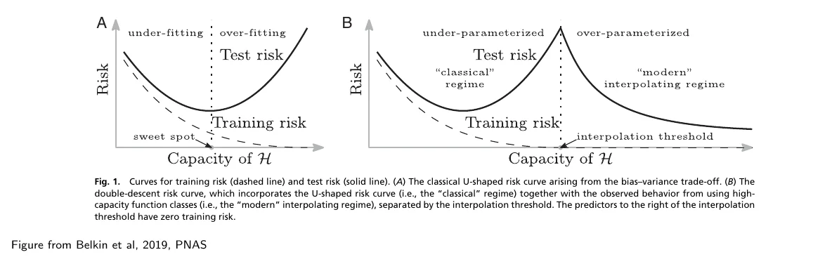
5. The excess risk splits into estimation error $R(f_n)-R(\tilde{f})$ (random, grows with the size of $\mathcal{F}$) and approximation error $R(\tilde{f})-R(f^{\ast })$ (deterministic, shrinks with the size of $\mathcal{F}$). Classical regime: U-shaped test risk. Modern regime: interpolation, double descent. For the $L_2$ loss, pointwise: $E(f_n(x)-f^{\ast }(x){)}^2=\text{variance}+{\text{bias}}^2$.
6. No Free Lunch: averaged over all possible true functions, all classifiers perform the same. Machine learning without an inductive bias is impossible.

Exam relevance

• Multiple choice (task 1 of the real exam, task 2 of the mock): what consistency means and what it does not mean, universal consistency (kNN), which error term is random, over- vs. under-parameterization, what NFL does and does not say. The mock asked exactly such statements; see the MC block below.
• Table tasks: empirical risks from a small sample, the ERM choice, estimation and approximation error from given true risks, bias and variance from a few predictions. Worked examples: ERM task, bias-variance task, NFL task.
• Sheet 2, Exercise 2 is the NFL on $\{0,1{\}}^4$ (kNN vs. memorize-or-zero, averaged over all $2^{16}$ target functions).

Overview: 1. The finite sample setting and consistency, 2. Estimating the risk by the empirical risk, 3. Empirical risk minimization and why it can fail, 4. Estimation and approximation error, 5. The bias-variance decomposition, 6. The No-Free-Lunch theorem.

Predicting in the finite sample setting

Finite sample setting and the training data

Slides 105-108

So far we discussed the “optimistic” regime in which we know the underlying distribution: then there is nothing to learn. Now we turn to the standard machine learning setting: we do not know the distribution, but we see samples from it (Bach Sec. 2, Devroye et al. Sec. 2, Hastie et al. Sec. 2.4-2.9). Everything we do has an attached uncertainty that depends on how well the sample represents $P$.

Training data

We draw $n$ training points $(X_i,Y_i{)}_{i=1,\dots ,n}\in \mathcal{X}\times \mathcal{Y}$ i.i.d. (independent and identically distributed) according to $P$.

The i.i.d. assumption makes a lot of sense in many cases (to some degree even for blocks of text in language model pre-training), and it lets us use many tools from statistics. But it is a strong assumption in many applications: time series (today’s weather depends on yesterday’s), patients from the same hospital or family, repeated measurements of the same person. A second issue the framework does not cover: different train and test distributions (a model trained on data from one hospital, used in another).

The goal of machine learning

Slide 109

Goal

Given $n$ training points, construct a function $f_n$ whose true risk is close to the Bayes risk: $R(f_n)\approx R^{\ast }$.

$f_n$ depends on the random sample, so $R(f_n)$ is a random variable. To make “close” precise we need convergence of random variables.

Recap: convergence of random variables

Slide 110

Three modes of convergence

Let $(U_i{)}_{i\in \mathbb{N}}$ be random variables and $U$ a random variable. $U_i$ converges to $U$

• in probability if $\forall \epsilon >0:{\lim }_{i\to \infty }P(|U_i-U|>\epsilon )=0$
• almost surely (a.s.) if $P({\lim }_{i\to \infty }{U}_i=U)=1$
• in $L_1$ / in expectation if ${\lim }_{i\to \infty }E(|U_i-U|)=0$

Almost sure convergence implies convergence in probability, $L_1$ convergence implies convergence in probability, and there are no other implications in general.

Consistency of a learning algorithm

Slides 111-113

Consider an infinite sequence of data points $(X_i,Y_i{)}_{i\in \mathbb{N}}$ drawn i.i.d. from $P$, and let $f_n$ be the function the algorithm $\mathcal{A}$ constructs from the first $n$ points.

Consistency

• $\mathcal{A}$ is consistent (for $P$) if the risk of $f_n$ converges to the Bayes risk in probability:

$$\forall \epsilon >0:\underset{n\to \infty }{\lim }P(R(f_n)-R^{\ast }>\epsilon )=0$$

• With almost sure convergence instead, $\mathcal{A}$ is strongly consistent.
• $\mathcal{A}$ is universally consistent if it is consistent for all distributions $P$ on $\mathcal{X}\times \mathcal{Y}$.

Universal consistency

No matter what the distribution is, after “enough data points” the true risk of $f_n$ is arbitrarily close to the best possible risk. This is what we ultimately want.

What consistency does not say

• It is about the convergence of the risk $R(f_n)\to R^{\ast }$, not about the function: $f_n$ need not converge to $f^{\ast }$ (pointwise or otherwise). Two very different functions can have the same risk.
• It is an asymptotic statement. It gives no rate: how many points are “enough” depends on $P$, and for every fixed $n$ there are distributions for which $R(f_n)$ is still far from $R^{\ast }$.

For a long time it was unknown whether universally consistent algorithms exist at all. The first positive answer came in 1977, when Stone proved that the kNN classifier is universally consistent (with $k\to \infty$ and $k/n\to 0$; with a fixed $k$, for example $k=1$, the noise of the nearest neighbour’s label never averages out). Since then, many algorithms have been shown to be universally consistent: support vector machines, boosting, random forests and more. Understanding the principles behind such results is a large part of this course.

Why not use the plug-in classifier and be done?

Slide 114

Idea: estimate the regression function $\eta (x)$ by some ${\eta }_n(x)$ from the training data and plug it into the Bayes classifier:

$$f_n(x):=\{\begin{array}{ll}1& \text{if }{\eta }_n(x)\ge 0.5\\ 0& \text{otherwise}\end{array}$$

• In theory: with a suitable estimator ${\eta }_n$, the plug-in approach is universally consistent. ☺
• In practice: estimating densities is notoriously hard, in particular in high-dimensional input spaces. We would need a ridiculous amount of training data, so the plug-in approach is useless in practice. ☹

Estimating the true risk by the empirical risk

Empirical risk

Slides 115-118

We defined the best classifier as the one that minimizes the true risk. Without $P$ we cannot compute the true risk. The obvious idea: estimate the risk from the sample and pick the function with the smallest estimated risk. The big question is whether this is (always? sometimes?) successful. First we look at how to estimate the risk of a fixed, given function $f$.

Empirical risk

$$R_n(f):=\frac{1}{n}\sum _{i=1}^n\ell (X_i,Y_i,f(X_i))$$

It can be computed from the training points alone. For the 0-1 loss it is the fraction of misclassified training points.

Is it a “good” estimate? A formal way to say this: $R_n(f)$ converges to $R(f)$ as $n\to \infty$.

Recap: law of large numbers

Slides 119-121

Proposition 5 (law of large numbers, simplest version)

Let $(Z_i{)}_{i\in \mathbb{N}}$ be independent random variables drawn from a distribution with expectation $E(Z)$. Then (under mild assumptions)

$$\frac{1}{n}\sum _{i=1}^n{Z}_i\to E(Z)\text{(almost surely)}$$

Mini example: why independence is crucial

Let $X_1$ be the toss of a fair coin and $X_2,X_3,\dots$ identical copies of $X_1$. Each $X_i$ is $\mathrm{Ber}(0.5)$ with $E(X_i)=0.5$, but they are not independent. Depending on $X_1$, the empirical average is always 0 or always 1, so it never converges to $0.5$.

“Mild assumptions”: there are many versions of the LLN. Often it is stated for random variables with finite variance, which makes the proof much simpler, but it also holds as long as the expectation exists. The $Z_i$ do not even need to be identically distributed, as long as they have the same expectation.

Convergence of the empirical risk of a fixed function

Slides 122-124

Proposition 6 (empirical risk converges for a fixed function)

In the standard setup, fix a function $f_0:\mathcal{X}\to \mathcal{Y}$. Then for this fixed $f_0$

$$R_n(f_0)\to R(f_0)\text{(almost surely)}$$

Proof

Apply the law of large numbers to $Z_i:=\ell (X_i,Y_i,f_0(X_i))$. These are independent (the points are i.i.d. and $f_0$ does not depend on them), with $E(Z_i)=R(f_0)$. $\square$

What it means, and what not

• For each fixed function, the training error is a good estimate of the test error when $n$ is large.
• It says nothing about how fast (no rate), and nothing about a function that was chosen using the data. That is exactly what a learning algorithm does, and it is the limitation that the next sections run into.

Empirical risk minimization

The ERM principle

Slides 125-127

For a fixed $f$, the empirical risk converges to the true risk. So to find $f^{\ast }$ (which minimizes the true risk), it makes sense to pick the function that minimizes the empirical risk and hope that it is close.

Empirical risk minimization (ERM)

• Define a set $\mathcal{F}$ of functions $\mathcal{X}\to \mathcal{Y}$.
• Choose a function with the smallest empirical risk:

$$f_n:=\underset{f\in \mathcal{F}}{\mathrm{argmin}}{R}_n(f)$$

It might not be unique. For simplicity we assume the minimizer exists (otherwise one argues with a sequence approaching the infimum).

The function class $\mathcal{F}$ is the important “parameter” of ERM: all linear functions, all decision trees of depth 5, all random forests, all two-layer MLPs, …

”Classical” regime vs. “modern” regime

Slide 128

Two regimes

• Classical regime: the function class $\mathcal{F}$ does not allow for interpolation.
• Modern regime / interpolation regime: $\mathcal{F}$ is so large that the training data can be interpolated (fitted with training error 0).

Is ERM always successful?

Slides 129-132

In our framework, a “successful” classifier is a consistent one. So: does ERM always converge?

Counterexample (slide 130)

• $\mathcal{X}=[0,1]$ with the uniform distribution. Labels are deterministic: $y=-1$ for $x<0.5$ and $y=+1$ for $x\ge 0.5$.
• Draw $n$ training points. Define $f_n$: on the training points, predict the training label; on all other points, predict $-1$.
• Then $R_n(f_n)=0$ but $R(f_n)=0.5$ for all $n$ (the set of training points has probability 0, so $f_n$ predicts $-1$ almost everywhere and is wrong on the right half).
• With $Z_i:=\ell (f_n(X_i),Y_i)$: $S_n={\sum }_i{Z}_i/n=0$ always, but $E(S_n)=0.5$.

Why can’t we use the LLN? The key property in the LLN is independence. Here $Z_i:=\ell (f_n(X_i),Y_i)$, but $f_n$ depends on all data points $(X_i,Y_i{)}_{i=1,\dots ,n}$. So even though the points are independent, the $Z_i$ are not: they all depend on $f_n$.

Trap

Slide 129 writes the question as ”$R_n(f_n)-R(f_n)\to 0$?“. This is the gap between training and test error of the selected function. The consistency question is $R(f_n)\to R^{\ast }$. In the counterexample both fail: the gap stays $0.5$, and $R(f_n)=0.5>R^{\ast }=0$.

Preview: statistical learning theory

It is not true that the minimizer of the empirical risk always converges to the Bayes classifier. Is machine learning doomed? No: statistical learning theory (Lecture 3) gives conditions on $\mathcal{F}$ under which ERM works after all.

ERM in practice

Slide 133

• Conceptually, ERM is a straightforward learning principle. The key to its success or failure is choosing a “good” function class $\mathcal{F}$: explicitly (classical regime) or implicitly (interpolation regime, sometimes).
• Computationally it can be hard: finding the minimizer of the 0-1 loss is often NP hard. This is why in practice we use convex relaxations of the 0-1 loss: the surrogate losses of Lecture 1.1.

Estimation and approximation error

Definitions

Slides 134-135

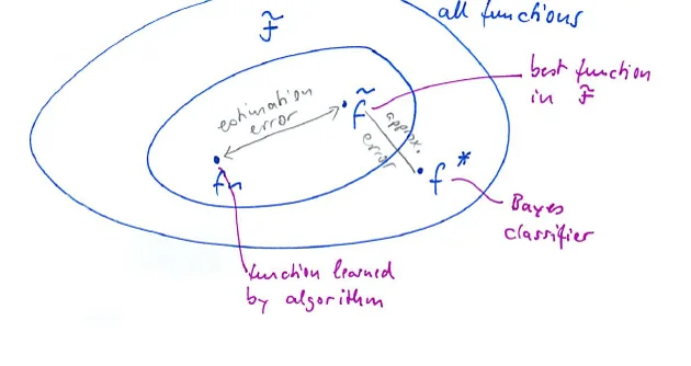
When we perform ERM we can make two types of error. Let $\tilde{f}:={\mathrm{argmin}}_{f\in \mathcal{F}}R(f)$ be the true best function in $\mathcal{F}$.

Estimation and approximation error

• Estimation error $R(f_n)-R(\tilde{f})$: a random variable that depends on the sample.
• Approximation error $R(\tilde{f})-R(f^{\ast })$: a deterministic quantity that does not depend on the sample, only on the choice of $\mathcal{F}$.

Decomposition of the excess risk

$$R(f_n)-R^{\ast }=\underset{\text{estimation error}}{\underbrace{R(f_n)-R(\tilde{f})}}+\underset{\text{approximation error}}{\underbrace{R(\tilde{f})-R(f^{\ast })}}$$

Slide 135: estimation error inside 𝓕, approximation error from 𝓕 to the Bayes classifier.

Task: ERM, estimation and approximation error

Exam-style task: ERM on a small sample (4 P)

$X$ is uniform on $\{1,2,3,4\}$ with $\eta (x)=P(Y=1\mid X=x)$ given below. $\mathcal{F}=\{f_2,f_3,f_4\}$ with threshold classifiers $f_t(x)=1$ iff $x\ge t$. The training sample $(x_i,y_i)$ is

$$(1,0),(1,0),(2,1),(2,1),(3,1),(3,0),(4,1),(4,1)$$

$x$	1	2	3	4
$\eta (x)$	0.1	0.6	0.3	0.9

(a) (1 P, easy) Compute $R_n(f)$ for all $f\in \mathcal{F}$ (0-1 loss). Which function does ERM select?

(b) (1.5 P, harder) Compute the true risks, $R^{\ast }$, and the estimation and approximation error of ERM.

(c) (1.5 P, transfer) Now let $\mathcal{F}$ be all functions $\{1,2,3,4\}\to \{0,1\}$. What happens to the approximation error, and what can happen to the estimation error?

Solution

(a) $f_2$ predicts 1 on $\{2,3,4\}$: one error at $(3,0)$, $R_n=1/8$. $f_3$: errors at both $(2,1)$ and at $(3,0)$, $R_n=3/8$. $f_4$: errors at both $(2,1)$ and at $(3,1)$, $R_n=3/8$. ERM selects $f_n=f_2$. (1 P)

(b) $R(f)=\frac{1}{4}{\sum }_x(1_{f(x)=1}(1-\eta (x))+1_{f(x)=0}\eta (x))$: $R(f_2)=\frac{1}{4}(0.1+0.4+0.7+0.1)=0.325$, $R(f_3)=\frac{1}{4}(0.1+0.6+0.7+0.1)=0.375$, $R(f_4)=\frac{1}{4}(0.1+0.6+0.3+0.1)=0.275$. The Bayes classifier predicts 1 on $\{2,4\}$ (where $\eta >0.5$): $R^{\ast }=\frac{1}{4}(0.1+0.4+0.3+0.1)=0.225$ (0.5 P). $\tilde{f}=f_4$. Approximation error $0.275-0.225=0.05$, estimation error $R(f_2)-R(f_4)=0.05$. (1 P) Note that $R_n(f_n)=0.125$ is far too optimistic.

(c) The Bayes classifier is now in $\mathcal{F}$, so the approximation error is 0 (0.5 P). ERM predicts 0 at $x=1$, 1 at $x=2$ and $x=4$; at $x=3$ the sample has one 1 and one 0, a tie. If ERM picks 1 there, $R(f_n)=0.325$ and the estimation error is $0.1$; if it picks 0, it finds the Bayes classifier. Both have $R_n=1/8$: a larger class lowers the approximation error, but the training error can no longer tell good and bad functions apart. (1 P)

The classical regime

Slides 136-138

In the classical regime, $\mathcal{F}$ is reasonably small (no interpolation). Then the two errors behave in opposite ways as $\mathcal{F}$ grows:

Slide 136: which one is which? The decreasing curve is the approximation error, the increasing one the estimation error. The true risk (their sum plus R*) is U-shaped.

Slide 137: true function quadratic, 𝓕 = linear functions (red, underfitting) or all polynomials (blue, overfitting).

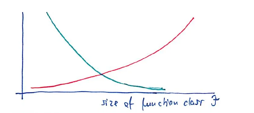
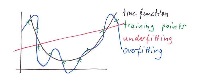
Overfitting and underfitting (classical regime)

• Overfitting: $\mathcal{F}$ is very large, so some $f\in \mathcal{F}$ explains all training points very well or exactly. Such a function tends to be complicated and models the noise as well, so predictions for unseen points are poor (large test error). Low approximation error, high estimation error.
• Underfitting: the model is too simple, $\mathcal{F}$ is too small. The estimated functions are stable with respect to noise, but cannot represent the truth. Large approximation error, low estimation error.

The modern regime and double descent

Slides 139-141

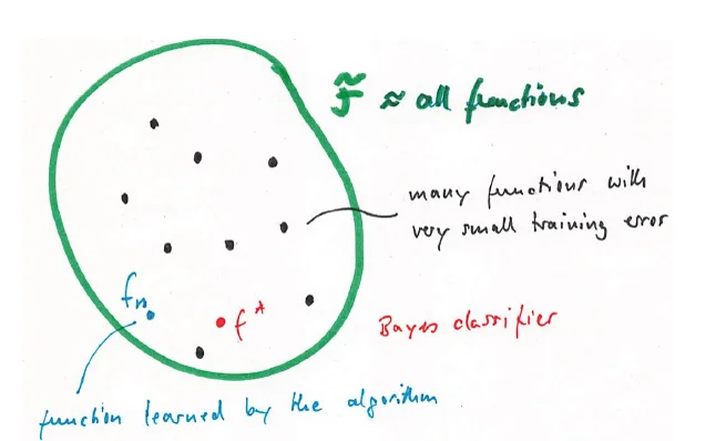
In the modern regime the function class is huge and covers pretty much all possible functions.

• The empirical risk minimizer interpolates the training points ($f_n$ has training error 0).
• The approximation error is often close to 0: the functions can represent almost anything.
• Traditional reasoning predicts a huge estimation error because of overfitting.
• But some algorithms always find solutions that interpolate and generalize well; these have a small estimation error. Practice shows that overfitting can even be beneficial.

There exist many functions with training error close to 0. Most of them would not generalize, some might. The question is how to find those.

Slide 139: modern regime, 𝓕 ≈ all functions.

Slide 141: the classical U-curve (A) and the double descent curve (B). Figure from Belkin et al., PNAS 2019.

Double descent

Below the interpolation threshold the classical picture holds. At the threshold the model is just able to fit the data and the test risk peaks. Beyond it, in the over-parameterized regime, the test risk falls again, often below the classical sweet spot. Why this can work is the topic of Lecture 8.

The bias-variance decomposition

Bias-variance tradeoff in L2 regression

Slides 142-147

Another decomposition of the error is most simple for regression with the squared loss. Let $f_n$ be constructed from $n$ random sample points and $f^{\ast }:{\mathbb{R}}^d\to \mathbb{R}$ the regression function. For a fixed point $x$, with the expectation over the random draw of the sample:

Bias-variance decomposition

$$E\left(\right(f_n(x)-f^{\ast }(x){)}^2)=\underset{\text{variance term}}{\underbrace{E\left(\right(f_n(x)-E(f_n(x)){)}^2)}}+\underset{\text{bias term}}{\underbrace{(E(f_n(x))-f^{\ast }(x){)}^2}}$$

• Variance term: the variance of the random variable $f_n(x)$.
• Bias term: how much $E(f_n)$ and $f^{\ast }$ deviate.

For every loss we have "$\le$" in this spirit, but for the $L_2$ loss we get equality (as in Proposition 3).

Proof

Add and subtract $E(f_n(x))$ inside the square (all expectations over the sample, $x$ fixed):

$$\begin{array}{rl}E((f_n(x)-f^{\ast }(x){)}^2)& =E\left(\right(f_n(x)-E{f}_n(x)+E{f}_n(x)-f^{\ast }(x){)}^2)\\ & =E((f_n(x)-E{f}_n(x){)}^2)+(E{f}_n(x)-f^{\ast }(x){)}^2\\ & +2E\left(\right(f_n(x)-E{f}_n(x)\left)\right(E{f}_n(x)-f^{\ast }(x)\left)\right)\end{array}$$

In the last term, $E{f}_n(x)-f^{\ast }(x)$ is deterministic and can be pulled out of the expectation. What remains is $E(f_n(x)-E{f}_n(x))=E{f}_n(x)-E{f}_n(x)=0$ by linearity. $\square$

Intuition

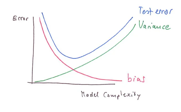
• Variance has the same intuition as the estimation error: it depends on the random data and on the capacity of $\mathcal{F}$.
• Bias has the same intuition as the approximation error: it does not depend on the data, only on the capacity of $\mathcal{F}$.

The classical picture (slide 147): as model complexity grows, the bias falls, the variance rises, and the test error is U-shaped.

Slide 147: the classical bias-variance figure.

The example of slide 137 as a simulation: noisy samples of a quadratic function, fitted by polynomials of degree d. The faint lines are fits to 30 different samples, their spread is the variance, the gap between their mean and the truth is the bias. Move the degree and the number of points.

Task: bias and variance from predictions

Exam-style task: bias and variance at one point (4 P)

An algorithm is trained on four independent training sets. At a fixed point $x_0$ it predicts $f_n(x_0)\in \{2.0,3.0,2.5,4.5\}$ (each with probability $1/4$). The true regression function is $f^{\ast }(x_0)=2$.

(a) (1 P, easy) Compute the bias term and the variance term.

(b) (1.5 P, harder) Verify the decomposition. Then use the shrunk predictor $g_n=0.5f_n$: bias, variance and expected squared error?

(c) (1.5 P, transfer) Which shrinkage factor $c$ minimizes the expected squared error of $c\cdot f_n$ at $x_0$? What does this say about bias and variance?

Solution

(a) $E{f}_n(x_0)=(2+3+2.5+4.5)/4=3$. Bias term $(3-2{)}^2=1$. Variance $\frac{1}{4}((-1{)}^2+0^2+(-0.5{)}^2+1.5^2)=\frac{3.5}{4}=0.875$. (1 P)

(b) Directly: $\frac{1}{4}(0^2+1^2+0.5^2+2.5^2)=\frac{7.5}{4}=1.875=1+0.875$ ✓ (0.5 P). For $g_n$: mean $1.5$, bias term $0.25$, variance $0.25\cdot 0.875=0.219$, total $0.469$: much better than $1.875$. (1 P)

(c) $\mathrm{MSE}(c)=(3c-2{)}^2+0.875c^2$. Setting the derivative $6(3c-2)+1.75c$ to 0 gives $c=12/19.75\approx 0.61$ and $\mathrm{MSE}\approx 0.354$. Shrinking adds bias but removes more variance. This is the idea of regularization (Lecture 5). (1.5 P)

The No-Free-Lunch theorem

Intuition and setup

Slides 148-151

(Presentation after Ho and Pepyne 2002; see also Shalev-Shwartz and Ben-David Sec. 5.1 and Devroye et al. Chapter 7.)

Intuition

There is no single best classifier that outperforms all other classifiers when averaged over all possible learning problems. There are many formal versions; the lecture uses the easiest one.

NFL setup

• The input space is a finite set $\mathcal{X}=\{x_1,\dots ,x_m\}$ with a fixed distribution, say uniform (the proofs work for all distributions).
• Binary classification, $\mathcal{Y}=\{\pm 1\}$, and the labels are deterministic functions of the input.
• There are $2^m$ functions $\mathcal{X}\to \mathcal{Y}$; call the set of all of them $\mathcal{F}$.
• One of them, $f^{\ast }$, is the true function; we observe noise-free training points $(x_i,f^{\ast }(x_i))$ and an algorithm estimates $f_n$.
• Table: rows are the estimated functions $f_i$, columns the true functions $f_j$, and the entry $r_{ij}$ is the true 0-1 error of $f_i$ when the true function is $f_j$.

With the uniform distribution, $r_{ij}$ is the fraction of points where $f_i$ and $f_j$ disagree.

Trap

The bullet text on slide 151 says “rows = true functions, columns = estimated functions”, the drawing and the definition of $r_{ij}$ use the other orientation. The statements below hold either way: they only count how many functions disagree with a given one on $k$ points.

Propositions 7 to 9

Slides 152-155

Proposition 7 (the risk in each row is the same)

In each row of the table, each risk value occurs the same number of times.

Proof

Fix a row $f_i$. Then $r_{ij}=0$ exactly once (when $f_j=f_i$), $r_{ij}=1/m$ exactly $m$ times (the functions that disagree with $f_i$ on one point), $r_{ij}=2/m$ exactly $\left(\genfrac{}{}{0ex}{}{m}{2}\right)$ times, and in general $r_{ij}=k/m$ exactly $\left(\genfrac{}{}{0ex}{}{m}{k}\right)$ times. These counts do not depend on $i$. $\square$

Proposition 8 (simple NFL)

On average over all true functions $f\in \mathcal{F}$, the performance of all classifiers $\hat{f}$ is the same.

Proof: obvious consequence of Proposition 7 (every row has the same multiset of values, so the same average).

Proposition 9 (simple NFL with training data)

Given a training set $(X_i,Y_i{)}_{i=1,\dots ,n}$: on average over all true functions that could have generated the training data, all estimated classifiers with 0 training error perform the same.

Proof

In the table, eliminate all columns that are not consistent with the training data. Among the remaining true functions, all labelings of the test points are possible, each exactly once. Every classifier with 0 training error agrees with them on the training points, and on the test points the same counting argument as in Proposition 7 applies. $\square$

The table of slide 151 for m = 3. Pick a true function and training points: inconsistent columns and rows with training errors fade out, and all remaining rows have the same average. Then switch on the inductive bias and watch the averages differ.

Task: No Free Lunch on three points

Exam-style task: NFL (4 P)

$\mathcal{X}=\{x_1,x_2,x_3\}$ with the uniform distribution, labels $\pm 1$. The only training point is $(x_2,+1)$. Classifier A predicts $+1$ everywhere. Classifier B predicts $+1$ at $x_2$ and $-1$ at $x_1$ and $x_3$. Write functions as label triples, for example $(+,+,-)$.

(a) (1 P, easy) List all true functions consistent with the training data.

(b) (1.5 P, harder) Compute the average true error of A and of B over these functions.

(c) (1.5 P, transfer) Assume the inductive bias “similar inputs, similar labels”: along $x_1,x_2,x_3$ the label changes at most once. Recompute the averages and explain the difference.

Solution

(a) $(+,+,+)$, $(+,+,-)$, $(-,+,+)$, $(-,+,-)$: the labels at $x_1$ and $x_3$ are free. (1 P)

(b) A $=(+,+,+)$ has errors $0,\frac{1}{3},\frac{1}{3},\frac{2}{3}$, average $\frac{1}{3}$. B $=(-,+,-)$ has errors $\frac{2}{3},\frac{1}{3},\frac{1}{3},0$, average $\frac{1}{3}$. Equal, as Proposition 9 says. (1.5 P)

(c) $(-,+,-)$ changes the label twice and is excluded. A: $0,\frac{1}{3},\frac{1}{3}$, average $\frac{2}{9}$. B: $\frac{2}{3},\frac{1}{3},\frac{1}{3}$, average $\frac{4}{9}$. Deleting columns breaks the symmetry of the table, and the classifier that matches the assumption wins. Without an assumption no classifier can be better; with one, some are. (1.5 P)

Discussion

Slides 156-159

We have seen that “the best possible classifier for all data sets” does not exist. Should we give up? Is machine learning meaningless?

No: machine learning needs an inductive bias

• In practice we do not consider all possible functions. As soon as we make assumptions on the function space (or even just exclude pathological functions), the NFL breaks down: assumptions restrict the set of possible true functions, which deletes columns from the table, and the proof breaks down.
• Example: a notion of similarity among the inputs $x_i$, and only functions that give similar labels to similar points. This excludes functions that look as if they distribute labels randomly.
• Machine learning without an inductive bias is impossible!

Much more general theorems exist, for example for data drawn from a joint distribution on $\mathcal{X}\times \mathcal{Y}$ with any space $\mathcal{X}$ (Wolpert 1996, Ho and Pepyne 2002, Devroye et al. Chapter 7).

The lecturer's question: why doesn't the NFL contradict universally consistent algorithms?

Universal consistency is an asymptotic statement for each fixed distribution: for every $P$, the risk converges to $R^{\ast }$ as $n\to \infty$. The NFL is a statement for a fixed training set size, averaged over all possible true functions. Both are true at the same time: for any fixed $n$ there are distributions on which a universally consistent algorithm is still bad (there is no uniform rate), but for each single distribution it eventually learns. In the finite NFL setting, once the training set covers all of $\mathcal{X}$, every consistent algorithm is perfect, and the NFL has nothing left to average over.

Summary

Concept	Definition	Key point
Consistency	$P(R(f_n)-R^{\ast }>\epsilon )\to 0$	about the risk, asymptotic, no rate
Universal consistency	consistent for every $P$	exists: kNN (Stone 1977), SVM, boosting, random forests
Empirical risk	$R_n(f)=\frac{1}{n}{\sum }_i\ell (X_i,Y_i,f(X_i))$	$\to R(f)$ for a fixed $f$ (LLN)
ERM	$f_n={\mathrm{argmin}}_{\mathcal{F}}{R}_n$	can fail: $f_n$ depends on the data
Estimation error	$R(f_n)-R(\tilde{f})$	random, grows with $\mathcal{F}$
Approximation error	$R(\tilde{f})-R^{\ast }$	deterministic, shrinks with $\mathcal{F}$
Variance / bias ($L_2$)	$E(f_n(x)-E{f}_n(x){)}^2$ / $(E{f}_n(x)-f^{\ast }(x){)}^2$	same intuition as estimation / approximation
No Free Lunch	averaged over all true functions, all classifiers equal	learning needs an inductive bias

Self-Test

Question cards (13)

What is the i.i.d. assumption, and where does it fail?

Answer

The training points $(X_i,Y_i)$ are drawn independently from the same distribution $P$. It fails for time series, grouped data (patients of one hospital, repeated measurements) and when train and test distributions differ.

Define consistency, strong consistency and universal consistency.

Answer

Consistent for $P$: $\forall \epsilon >0:P(R(f_n)-R^{\ast }>\epsilon )\to 0$. Strongly consistent: the same with almost sure convergence. Universally consistent: consistent for every distribution $P$.

Name two things consistency does not guarantee.

Answer

That $f_n$ converges to $f^{\ast }$ as a function (only the risk converges), and any rate: how large $n$ must be depends on $P$, and for every fixed $n$ there are distributions where $f_n$ is still bad.

Which algorithm was first shown to be universally consistent, and under which condition?

Answer

The kNN classifier (Stone 1977), with $k\to \infty$ and $k/n\to 0$. With a fixed $k$ (for example 1-NN) it is not universally consistent.

What is the plug-in classifier, and why is it useless in practice?

Answer

Estimate $\eta$ by ${\eta }_n$ and predict 1 iff ${\eta }_n(x)\ge 0.5$. It is universally consistent with a suitable estimator, but estimating densities in high dimensions needs a ridiculous amount of data.

State Proposition 6 and its proof. Why does it not show that ERM works?

Answer

For a fixed $f_0$, $R_n(f_0)\to R(f_0)$ a.s., by the LLN applied to $Z_i=\ell (X_i,Y_i,f_0(X_i))$. ERM selects $f_n$ using the data, so the $Z_i=\ell (X_i,Y_i,f_n(X_i))$ are no longer independent and the LLN does not apply.

Give the counterexample showing that ERM can fail.

Answer

$X$ uniform on $[0,1]$, $y=-1$ for $x<0.5$ and $+1$ otherwise. $f_n$ returns the training label on training points and $-1$ elsewhere: $R_n(f_n)=0$ but $R(f_n)=0.5$ for all $n$.

Why does one minimize surrogate losses instead of the 0-1 loss in practice?

Answer

Minimizing the empirical 0-1 loss is often NP hard. Convex relaxations (hinge, logistic, …) can be minimized efficiently and are classification-calibrated.

Define estimation and approximation error and say which one is random.

Answer

With $\tilde{f}={\mathrm{argmin}}_{\mathcal{F}}R$: estimation error $R(f_n)-R(\tilde{f})$ (random, depends on the sample), approximation error $R(\tilde{f})-R(f^{\ast })$ (deterministic, depends only on $\mathcal{F}$). They sum to the excess risk $R(f_n)-R^{\ast }$.

How do the two errors behave as $\mathcal{F}$ grows in the classical regime, and how does that relate to over- and underfitting?

Answer

The approximation error falls, the estimation error rises, the true risk is U-shaped. Underfitting: small $\mathcal{F}$, large approximation error, low estimation error. Overfitting: large $\mathcal{F}$, low approximation error, high estimation error.

What is different in the modern (interpolation) regime?

Answer

$\mathcal{F}$ is so large that ERM interpolates the training data and the approximation error is about 0. Classical reasoning predicts a huge estimation error, but some algorithms find interpolating solutions that generalize well; the test risk shows double descent beyond the interpolation threshold.

State and prove the bias-variance decomposition.

Answer

$E(f_n(x)-f^{\ast }(x){)}^2=E(f_n(x)-E{f}_n(x){)}^2+(E{f}_n(x)-f^{\ast }(x){)}^2$. Add and subtract $E{f}_n(x)$, expand; the cross term is $2(E{f}_n(x)-f^{\ast }(x))E(f_n(x)-E{f}_n(x))=0$.

State Propositions 7, 8 and 9 of the NFL and the main conclusion.

Answer

7: in each row of the error table each risk value $k/m$ occurs equally often ($\left(\genfrac{}{}{0ex}{}{m}{k}\right)$ times). 8: averaged over all true functions, all classifiers perform the same. 9: averaged over all true functions consistent with the training data, all classifiers with 0 training error perform the same. Conclusion: learning needs an inductive bias that excludes some true functions.

Multiple Choice

Multiple choice (8)

A learning algorithm is consistent for $P$. Which statement follows?

• $f_n(x)\to f^{\ast }(x)$ for almost every $x$.

• $P(R(f_n)-R^{\ast }>\epsilon )\to 0$ for every $\epsilon >0$.

• $R(f_n)-R^{\ast }\le C/\sqrt{n}$ for a constant $C$ that does not depend on $P$.

• The algorithm is consistent for every other distribution as well.

Explanation

Consistency is convergence in probability of the risk. It says nothing about the function itself, gives no distribution-free rate, and holds for this $P$ only (for all $P$ it would be universal consistency).

Which of the following is universally consistent?

• the 1-nearest-neighbour classifier

• ERM over the class of linear classifiers

• kNN with $k(n)\to \infty$ and $k(n)/n\to 0$

• the plug-in classifier with any estimator ${\eta }_n$

Explanation

Stone’s theorem. 1-NN never averages out the label noise; ERM over a fixed class converges at best to the best function in the class, which has an approximation error; the plug-in classifier needs a suitable estimator.

Why can the law of large numbers not be used to show $R_n(f_n)\to R(f_n)$ for the ERM solution $f_n$?

• because the loss is not bounded

• because the training points are not identically distributed

• because $f_n$ depends on all training points, so the losses $\ell (X_i,Y_i,f_n(X_i))$ are not independent

• because the empirical risk is not an average

Explanation

The training points are i.i.d., but the summands all depend on the data-dependent $f_n$. Independence is the key assumption of the LLN (compare the coin example of slide 120).

In the classical regime, the function class $\mathcal{F}$ is made larger. What typically happens?

• both the approximation and the estimation error decrease

• the approximation error decreases, the estimation error increases

• the approximation error increases, the estimation error decreases

• the Bayes risk decreases

Explanation

A larger class contains functions closer to $f^{\ast }$ (lower approximation error) but also more functions that fit the noise (higher estimation error). The Bayes risk depends only on $P$.

Which statement about the over-parameterized (interpolation) regime is true?

• The approximation error is large, because interpolating functions are complicated.

• Every interpolating function has a large test error.

• Some algorithms find interpolating solutions with a small estimation error.

• The test risk increases monotonically with the capacity beyond the interpolation threshold.

Explanation

In the modern regime the approximation error is about 0 and training error 0 is reached; many interpolating functions generalize badly, but some algorithms find ones that generalize well. Beyond the threshold the risk typically falls again (double descent).

In the bias-variance decomposition at a fixed point $x$, which quantity is not affected by the randomness of a single training sample, but only by the distribution of $f_n(x)$ as a whole and by $f^{\ast }$?

• the bias term $(E{f}_n(x)-f^{\ast }(x){)}^2$

• the prediction $f_n(x)$

• the squared error $(f_n(x)-f^{\ast }(x){)}^2$

• the deviation $f_n(x)-E{f}_n(x)$

Explanation

The bias is a deterministic number (like the approximation error). The other three are random variables that change with the sample; the variance term is the expectation of the squared last one.

Which statement does the simple No-Free-Lunch theorem (Proposition 9) make?

• Universally consistent algorithms cannot exist.

• Every classifier with training error 0 has test error 0.5.

• Averaged over all true functions consistent with the training data, all classifiers with training error 0 have the same error.

• kNN is better than any other classifier on average over all true functions.

Explanation

The NFL is an average over all possible true functions for a fixed training set. It does not contradict universal consistency (an asymptotic statement for each fixed $P$), and it does not say that a single classifier has error 0.5 on a given problem.

Which mode of convergence always implies convergence in probability?

• none of them, the three modes are unrelated

• almost sure convergence (and also $L_1$ convergence)

• only convergence in expectation of $U_i$, i.e. $E(U_i)\to E(U)$

• convergence in probability implies almost sure convergence

Explanation

Slide 110: a.s. ⇒ in probability and $L_1$ ⇒ in probability, no other implications in general. $E(U_i)\to E(U)$ is weaker than $L_1$ convergence $E|U_i-U|\to 0$.

References

All sources cited on the slides, in slide order (7 entries)

Slide	Source	Key point
106	Bach Sec. 2; Devroye et al. Sec. 2; Hastie et al. Sec. 2.4-2.9	reading for the finite sample setting
113	Stone, “Consistent Nonparametric Regression”, Annals of Statistics, 1977	kNN is universally consistent
141	Belkin, Hsu, Ma and Mandal, “Reconciling modern machine-learning practice and the classical bias-variance trade-off”, PNAS 2019	double descent curve
148, 158	Ho and Pepyne, “Simple explanation of the no-free-lunch theorem and its implications”, Journal of Optimization Theory and Applications, 2002	the NFL presentation of the lecture
148	Shalev-Shwartz and Ben-David, Understanding Machine Learning, Sec. 5.1 (online)	NFL, different formulation
148, 158	Devroye, Györfi and Lugosi, A Probabilistic Theory of Pattern Recognition, Chapter 7	more general NFL
158	Wolpert, “The Lack of A Priori Distinctions between Learning Algorithms”, Neural Computation, 1996	original general NFL

Related

• Previous: Lecture 1.1: Introduction and Decision Theory · Next: Lecture 2: Perceptron Mistake Bound · Course: Overview
• Concepts: Consistency, Empirical Risk Minimization, Estimation and Approximation Error, Bias-Variance Decomposition, No Free Lunch Theorem, Inductive Bias
• Exercises: Sheet 2, Exercise 2 (No Free Lunch on $\{0,1{\}}^4$), Exercise 1 (accuracy vs. loss)