Lecture 13: Forecasting AI Progress

TL;DR

1. Forecasting is measurable: a good forecaster maximizes sharpness subject to calibration; proper scoring rules (Brier, log score) reward reporting your true belief. Toolkit: decomposition, base rates, calibration training. Prediction markets are calibrated short-term but biased on long horizons.
2. The engine: loss follows scaling laws in compute, data and parameters; training compute grows 4-5×/year (far faster than Moore’s law), algorithms add ~3×/year, test-time compute is a second scaling axis, and unhobbling/overhangs give step changes that trend lines miss. A capability → product → revenue → compute flywheel drives it.
3. The ceiling is physical, the timing is bottlenecked: ~2×10²⁹ FLOP is likely feasible by 2030 (~5,000× GPT-4), bounded by power, chips (TSMC, CoWoS, HBM, ASML EUV) and capital. Moravec’s paradox and Amdahl’s law explain why the physical world and serial bottlenecks lag.
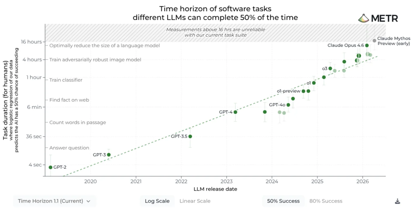
4. Measuring the trend: benchmarks saturate ever faster; experts and superforecasters underpredicted progress; METR time horizons double every ~7 months (since 2023 ~4), frontier at 12 to 17 h, but other domains lag.
5. Scenarios: the classical singularity, Bio-Anchors (median ~2050 → ~2040), Situational Awareness (automated researcher by 2027), AI 2027 (coder → ASI in ~1 year), the AI Futures Model (late 2020s to mid-2030s), Europe 2031, AI 2040 Plan A. A timeline is never only a timeline: it carries a view on whether the outcome is wanted.

Exam relevance

3 questions from this lecture (no mock exam question). Likely topics: calibration vs. sharpness, what makes a scoring rule proper, the Brier decomposition, the forecaster’s toolkit, the long-horizon problem of prediction markets, scaling laws, compute vs. algorithmic progress (4-5× and ~3× per year), test-time compute, unhobbling and overhangs, the constraints on scaling to 2030, Moravec’s paradox and Amdahl’s law, why benchmarks are a poor long-term ruler, the METR time horizon and its domain dependence, how Bio-Anchors / Situational Awareness / AI 2027 forecast and how they were revised.

Overview: I. The science of forecasting, II. The engine of progress, III. Measuring AI progress, IV. Future scenarios.

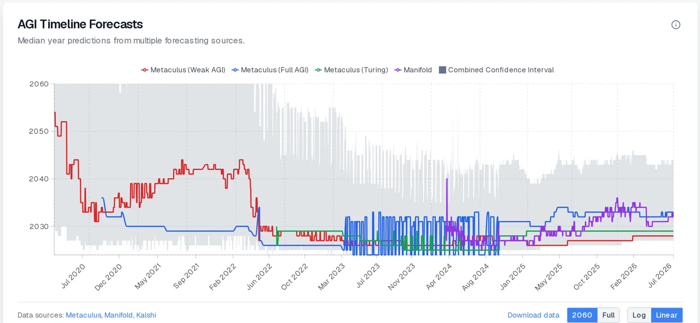
AGI Timelines Keep Moving

Slides 2-3

Slide 2: median AGI-year predictions from Metaculus (weak AGI, full AGI, Turing) and Manifold, 2020 to 2026. The medians fell from ~2050 to around 2030 after 2022, with a wide confidence band.

Part	Topic
I. The science of forecasting	how to make good forecasts; what is a “good” forecast?
II. The engine of progress	physics, Moore’s law, scaling laws, algorithmic progress
III. Measuring AI progress	benchmarks, the GPT series, METR task time horizons
IV. Future scenarios	from the classical singularity to Situational Awareness

Part I: The Science of Forecasting

Slide 4

Calibration and scoring.

What Makes a Good Forecaster

Slide 5

Calibration and sharpness

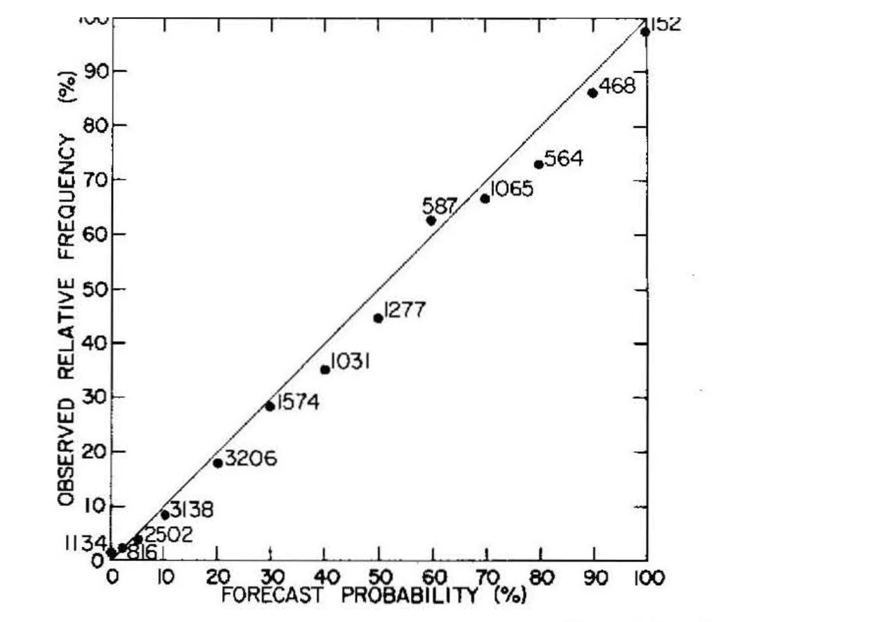
A forecaster is calibrated if, among all events assigned probability $p$, a fraction $p$ actually occur, for every $p$. Sharpness measures how concentrated (confident, far from the base rate) the forecasts are. The goal: maximize sharpness subject to calibration (Gneiting, Balabdaoui & Raftery, “Probabilistic Forecasts, Calibration and Sharpness”, JRSS-B 2007; Dawid, “The Well-Calibrated Bayesian”, JASA 1982).

A reliability diagram plots forecast probability (x) against observed frequency (y); points on the diagonal are calibrated.

Why both

Always predicting the base rate is perfectly calibrated but useless (no sharpness). Always saying 0% or 100% is maximally sharp but badly calibrated. A good forecaster is confident and right as often as claimed.

See Forecasting and Calibration.

Proper Scoring Rules

Slide 6

Brier score and Murphy's decomposition

The Brier score is the mean squared error of a probability forecast $f_i$ against the outcome $o_i\in \{0,1\}$:

$$\mathrm{BS}=\frac{1}{N}\sum _{i=1}^N(f_i-o_i{)}^2$$

Murphy’s decomposition (Murphy, J. Appl. Meteorology 1973) splits it into three parts:

$$\mathrm{BS}=\underset{\text{calibration gap}}{\underbrace{\text{Reliability}}}-\underset{\text{discrimination}}{\underbrace{\text{Resolution}}}+\underset{\text{base-rate entropy}}{\underbrace{\text{Uncertainty}}}$$

Lower is better: small reliability term (calibrated), large resolution (sharp, discriminating). Uncertainty depends only on the events.

Strictly proper

The log score $-\log p(\text{outcome})$ is strictly proper: the expected score is optimized only by reporting your true belief (Gneiting & Raftery, “Strictly Proper Scoring Rules”, JASA 2007). So a forecaster can’t gain by shading forecasts towards 0.5 or towards extremes.

Slide 6: a single Chicago weather forecaster, 1972-76. When a trained forecaster says "30% chance of rain", it rains about 30% of the time. More examples at calibration.city.

The Forecaster’s Toolkit

Slide 7

Worked example: “Will AI reach a 40-hour task horizon by the end of 2028?”

flowchart LR
  Q["Question<br/>40 h horizon by end of 2028?"] --> B["Base rate<br/>frontier now ~15 h at 50%"]
  Q --> R["Reference class<br/>doubling every ~4 to 7 months"]
  Q --> I["Inside-view adjustment<br/>data, capital, noise above 16 h?"]
  B --> E["Calibrated estimate<br/>55 to 70% Yes"]
  R --> E
  I --> E

1. Question decomposition: split one hard question into pieces you can actually estimate, then recombine into a single calibrated number.
2. Base rates first: anchor each piece to how often things like it happen, then adjust (the method of Tetlock & Gardner, “Superforecasting”, 2015).
3. Calibration training: log predictions and score them to learn your biases. Practice on Fatebook, Calibration and Pastcasting (by Sage). Background: LessWrong, “Forecasting & Prediction”.

”Making Beliefs Pay Rent”

Slide 8

A belief is only valuable if it has predictive power (Yudkowsky, “Making Beliefs Pay Rent (in Anticipated Experiences)”, 2007).

Pays rent	Floating belief
”the scaling trend holds” → METR horizon > 30 h during 2027; GPT-6 beats GPT-5 on a held-out benchmark; lab revenue keeps roughly 2×/year	”AI is a big deal” → “it is powerful” → “it is important”
every arrow is an observation that can be falsified	connects only to other statements, permits any experience

If no possible observation would change a belief, it is a floating belief that is not falsifiable.

Prediction Markets

Slide 9

Online platforms with contracts and resolution criteria to bid on future events (Wolfers & Zitzewitz, “Prediction Markets”, JEP 2004):

Platform	Type
Polymarket	real money (crypto)
Kalshi	real money, CFTC-regulated
Manifold	play money
Metaculus	not a market: aggregated individual forecasts, proper-scored

The long-horizon problem

Capital locked in a five-year contract forgoes market returns. This leads to a “no-trade region”, and long-shot dates are unreliable. Markets are well calibrated on two-week ranges and biased on fifteen-year ranges (“Can Interest-Bearing Positions Solve the Long-Horizon Problem in Prediction Markets?”, 2026). AGI-date markets are exactly the long-horizon kind.

Sidenote: How Good Is AI Itself at Forecasting?

Slide 10

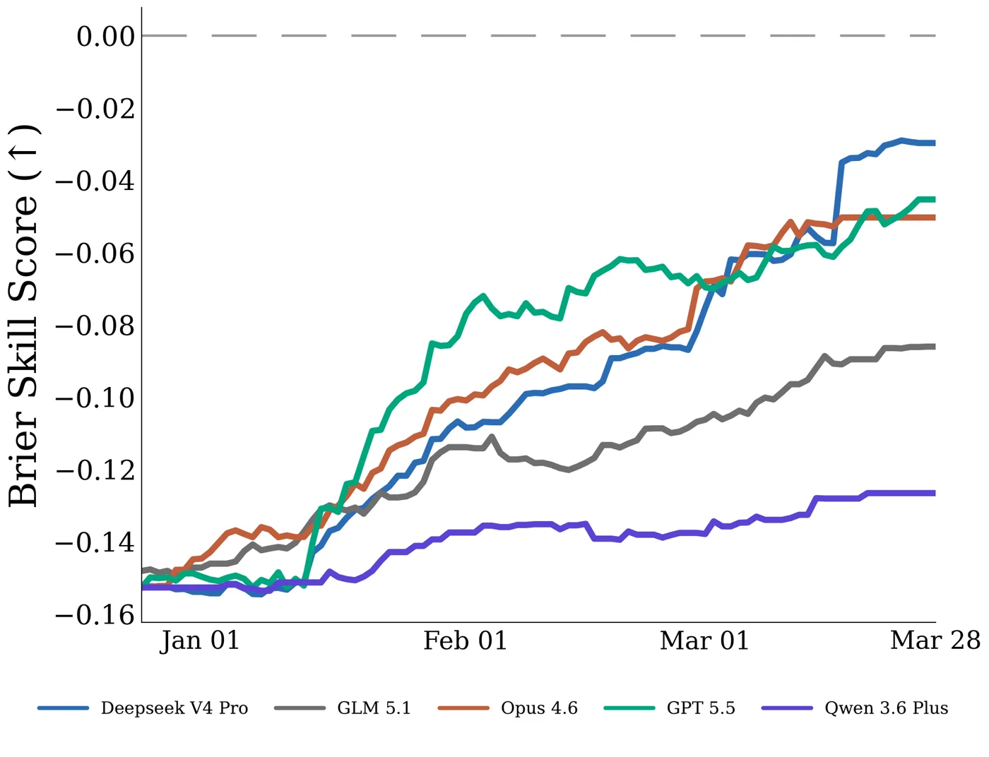
Goel et al., “FutureSim: Replaying World Events to Evaluate Adaptive Agents”, 2026 (arXiv:2605.15188) starts agents past their knowledge cutoff and replays the news day by day from January 2026. Models continuously predict 330 events that resolve over 88 days.

• Top-1 accuracy: GPT-5.5 25%, Opus 4.6 20%, then a gap to open-weight models (5 to 13%).
• Models improve over time, showing they can update their priors from new information. Calibration is still suboptimal.

Slide 10: FutureSim results. Source: Goel et al., 2026; see also the Forecasting Research Institute.

Part II: The Engine of Progress

Slide 11

Mechanisms that influence AI progress.

Deep Learning Capabilities Follow Scaling Laws

Slide 12

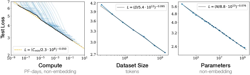
• Hestness et al., “Deep Learning Scaling is Predictable, Empirically”, 2017: power-law error curves across translation, language, vision and speech.
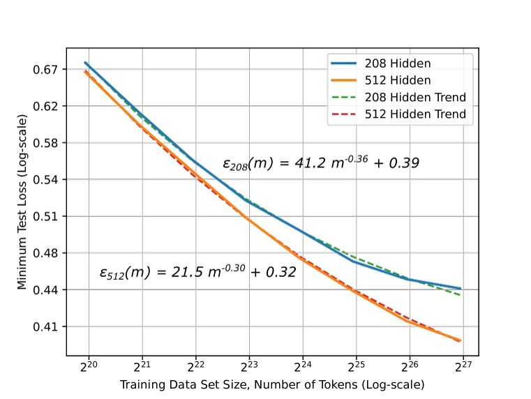
• Kaplan et al., “Scaling Laws for Neural Language Models”, 2020: loss falls as a power law in compute, data and parameters, over seven orders of magnitude.

Power law

$$L(C)\approx {\left(\frac{C_0}{C}\right)}^{\alpha }$$

A straight line on a log-log plot: every 10× more compute buys a fixed fraction off the loss. This is what makes progress extrapolable. See Scaling Laws and Training Compute.

Slide 12 (left): power-law generalization error vs. training set size. Source: Hestness et al., 2017.

Slide 12 (right): test loss vs. compute, dataset size and parameters. Source: Kaplan et al., 2020, Fig. 1.

Moore’s Law

Slide 13

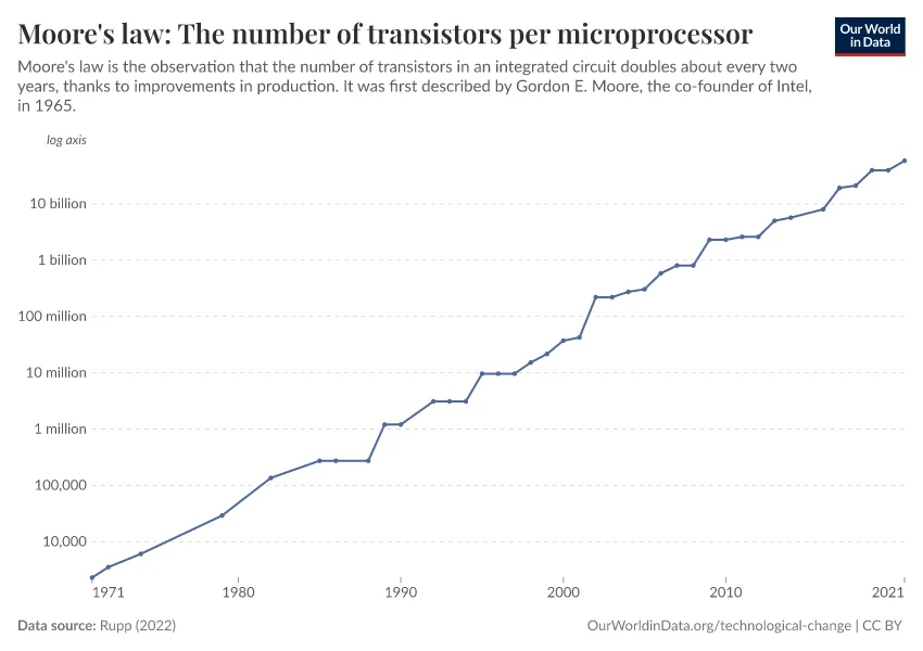
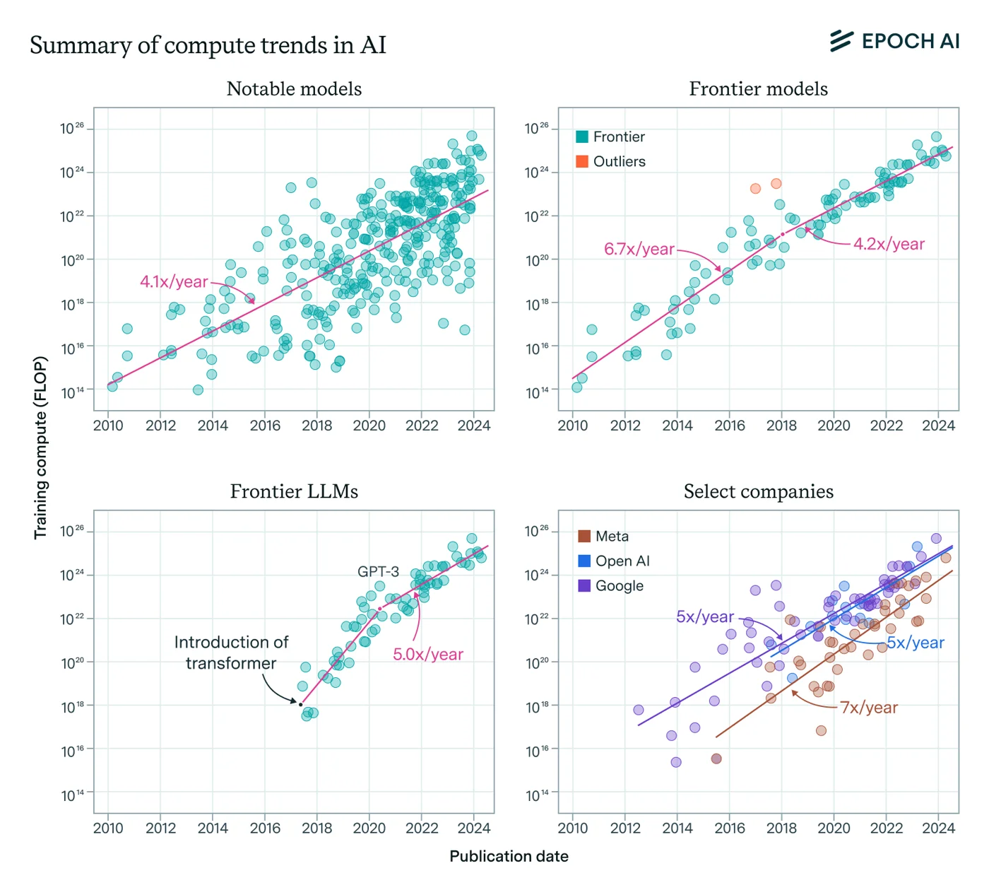
Transistor density doubles about every two years (Our World in Data, “Moore’s Law”). But AI compute outpaces Moore’s law by roughly an order of magnitude in exponent: frontier training compute grows 4-5× per year (Epoch AI). Current growth is mostly scaling of chip count (more chips, more spend), although chip density is a factor.

Slide 13 (left): Moore's law. Source: Our World in Data.

Slide 13 (right): training compute of frontier models grows 4-5× per year. Source: Epoch AI.

Algorithmic Progress as a Second Exponential

Slide 14

The compute needed to reach a fixed level of performance falls over time, from better architectures, optimizers and data quality:

Quantity	Value
halving time of compute-to-fixed-performance (language)	~8 months
algorithmic efficiency gain	~3×/year (faster than Moore’s law on its own)

Effective compute

Physical compute ~5×/year × algorithms ~3×/year ≈ ~15×/year effective compute for frontier models (Ho et al., “Algorithmic Progress in Language Models”, 2024). Over 2012 to 2023, compute contributed more than algorithms, but both compound. Vision shows the same pattern (Erdil & Besiroglu, 2022; Epoch AI Trends).

Test-Time Compute: A Second Scaling Axis

Slide 15

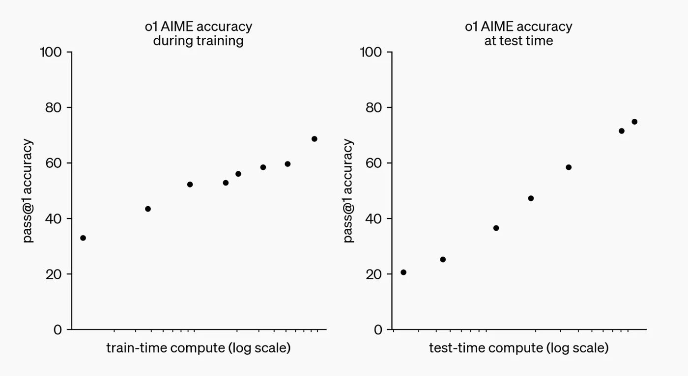
OpenAI’s o1 (Sept 2024) showed accuracy rising with compute spent at inference, not only in training. On AIME, GPT-4o scored 12%, o1 up to 83% (OpenAI, “Learning to Reason with LLMs”, 2024; Muennighoff et al., “s1: Simple Test-Time Scaling”, 2025).

Epoch: reasoning-training compute scaled ~10× from o1 to o3, then converges to the base ~4×/year trend within about a year (Epoch, “How far can reasoning models scale?”). A new axis gives a one-off jump, then joins the general trend. Background in RLVR.

Slide 15: accuracy rises with compute at training (left) and at inference (right). Source: OpenAI, 2024.

Unhobbling and Overhangs

Slide 16

Some capability gains are surprising and not predictable by scaling (Aschenbrenner, “Situational Awareness”, 2024):

Mechanism	Meaning	Example
Unhobbling	features that make existing models usable	RLHF, chain-of-thought (~10× effective compute on reasoning), scaffolding, tools, context length
Hardware overhang	capability latent in existing chips, unlocked by a new method	using GPUs for deep learning in 2012
Software overhang	a model whose full ability is only elicited later by better prompting or scaffolds	Claude Code

Key point

Overhangs are why trend extrapolation tends to undershoot around a paradigm shift: the straight line on the compute axis misses the step change when a latent capability is unlocked.

AI Progress as an Extension of Economic Growth

Slide 17

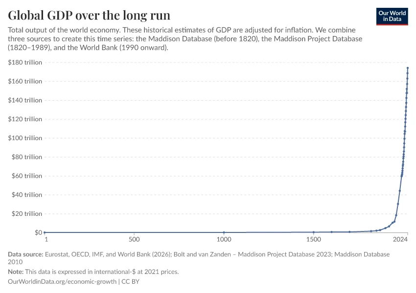
World output was nearly flat for most of history, then bent sharply upward with industrial capitalism. AI compute spending is the newest term in that series. The optimistic case for continued scaling: AI is the next phase of this curve.

Slide 17: two centuries of compounding economic growth. Source: Our World in Data, "Economic Growth" (Maddison Project data).

Can Scaling Continue to 2030?

Slide 18

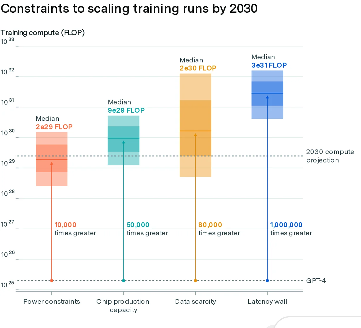
Sevilla et al., “Can AI Scaling Continue Through 2030?”, Epoch AI, 2024 estimates feasible 2030 training-run sizes under four constraints (power, chip manufacturing, data, latency). Conclusion: about 2 × 10²⁹ FLOP is likely feasible by 2030, roughly 5,000× GPT-4.

Slide 18: feasible 2030 training-run sizes under four constraints. Source: Sevilla et al., Epoch AI, 2024.

Electricity

Slide 19

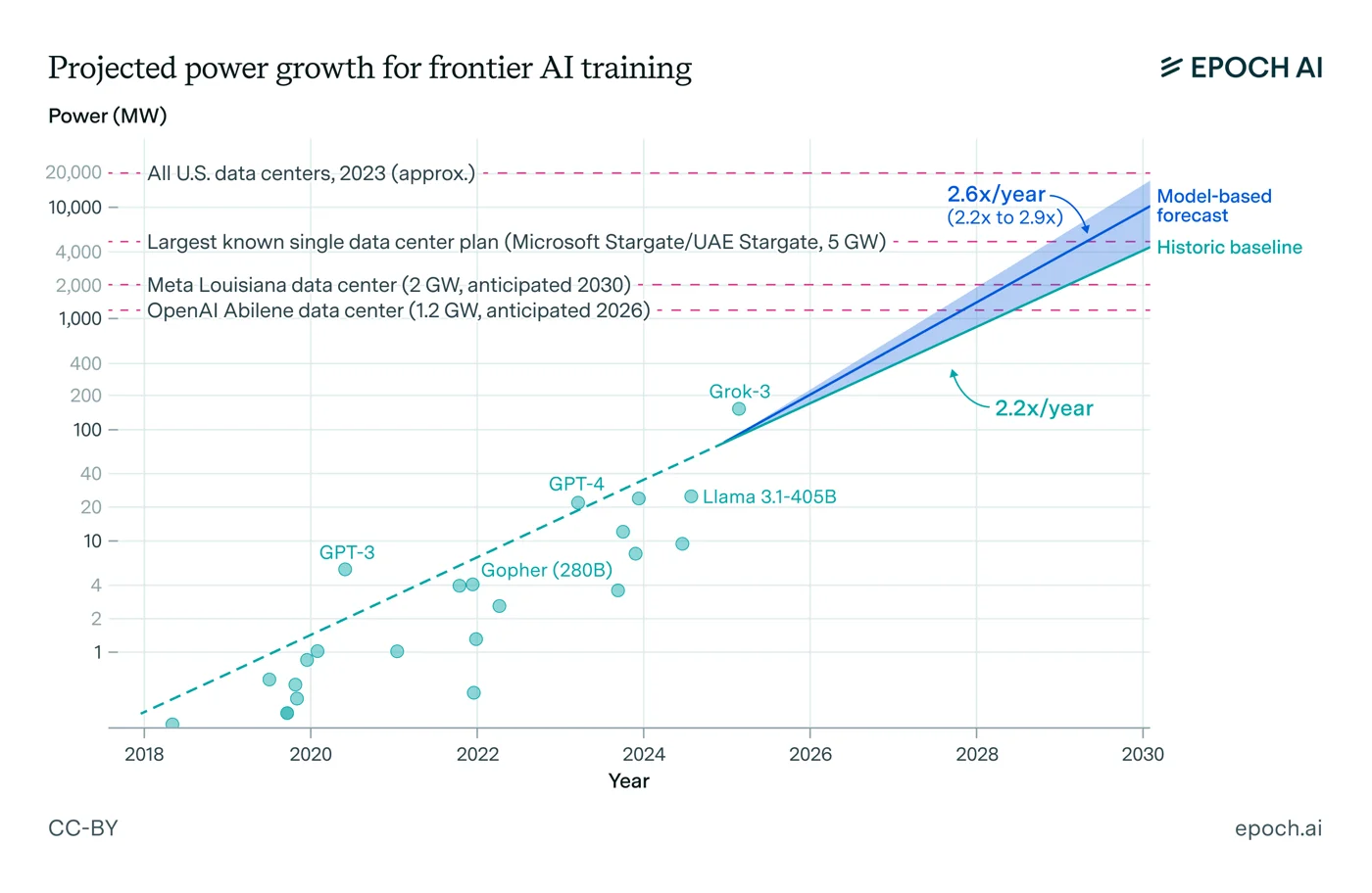
Frontier training sites reached about 1 GW in 2026. Five such sites are online: Anthropic-Amazon, xAI Colossus 2, Microsoft Fayetteville, Meta Prometheus, OpenAI Stargate Abilene (Epoch AI, Frontier Data Centers Hub).

• US datacenter power: ~31 GW (2025) heading towards ~66 GW (2027).
• By 2030, datacenters could draw 9 to 17% of US electricity.
• Grid interconnection and transformer supply are real limits. Hyperscalers are signing nuclear and gas deals directly.

Slide 19: per-training-run power on a log axis; the frontier crosses the gigawatt reference lines before 2030. Source: Epoch, "Power demands of frontier AI training".

The Chip Chokepoint: TSMC and Taiwan

Slide 20

• TSMC holds about 72% of foundry revenue and over 90% of leading-edge production. Almost all 2nm and most 3nm is in Taiwan through 2026 and 2027 (CSIS, “Taiwan’s Semiconductor Dominance”).
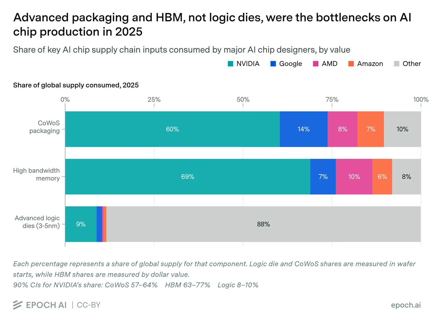
• New bottlenecks: advanced packaging (CoWoS) and high-bandwidth memory (HBM). The four big AI designers used ~12% of advanced logic, but ~90% of CoWoS and ~90% of HBM by value. Both were sold out into 2027 (Epoch AI, “AI chip supply chain constraints”).

Slide 20: AI chip supply-chain constraints. Source: Epoch AI.

Where Do Wafers Come From?

Slide 21

Extreme-ultraviolet (EUV) lithography is what makes sub-7nm chips possible. One company builds the machines: ASML, in Veldhoven, the Netherlands.

• About 48 EUV systems shipped in 2025, with 60 or more guided for 2026 (ASML Q4 2025 results).
• China has never received an EUV machine (export controls since ~2019). SMIC is stuck at 7nm and 5nm on older DUV lithography.

One company, one country, one town

The entire frontier uses sixty machines a year. This is currently Europe’s only point of leverage in the AI supply chain.

Summary: The Toolchain for Continued Scaling

Slide 22

If LLMs are a general method that keeps scaling with compute (Sutton, “The Bitter Lesson”, 2019), the compute chain is:

flowchart LR
  Z["Zeiss optics<br/>EUV mirrors (DE)"] --> A["ASML EUV<br/>lithography (NL)"] --> T["TSMC fabs<br/>Taiwan"] --> N["NVIDIA GPUs<br/>accelerators"] --> C["AI companies<br/>capital, datacenters"] --> F["Frontier model"]
  H["HBM / DRAM<br/>Korea"] --> N
  P["Power transformers<br/>+ electricity (GW)"] --> C
  G["Algorithmic progress<br/>~3x per year?"] --> F

Every link is concentrated in very few firms or countries, so each is a possible brake.

Frontier Company Capitalization

Slide 23

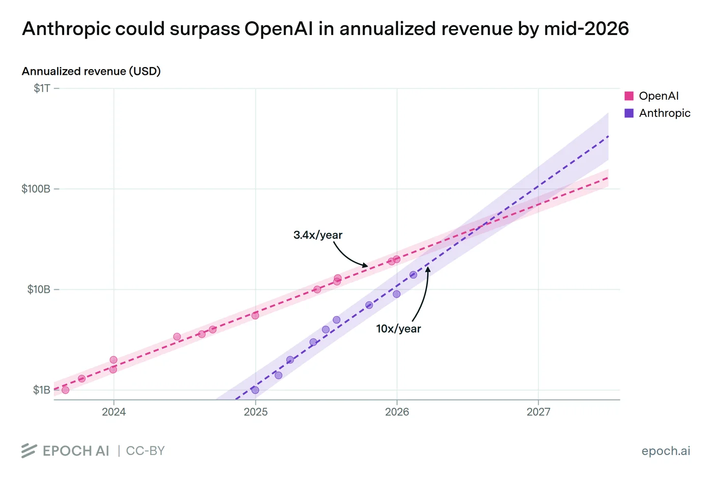
Frontier-lab revenue is real and growing fast. Whether it grows fast enough is the open question.

• 2026 hyperscaler capital spending is about $700B, roughly double 2025. OpenAI has committed on the order of $1.4 trillion in future compute against roughly $25B of current revenue.
• Forecasters underestimated revenue most of all: $16B predicted for 2025 vs. about $30B actual (Epoch, “How well did forecasters predict 2025 AI progress?”).
• The Bank for International Settlements warned of bubble risk in June 2026. A survey found 90% of firms report no productivity impact yet.

Slide 23: Epoch AI, Anthropic vs. OpenAI revenue. Revenue accounting is contested.

Warning

If the revenue leg can’t keep pace with capital expenditure, the flywheel stalls, and the compute trend bends well before physical constraints.

Moravec’s Paradox

Slide 24

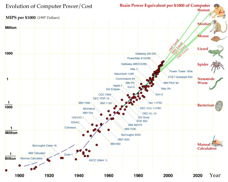
Hans Moravec, Mind Children, 1988

“It is comparatively easy to make computers exhibit adult level performance on intelligence tests or playing checkers, and difficult or impossible to give them the skills of a one-year-old when it comes to perception and mobility.”

(Moravec, “Mind Children”, Harvard UP 1988.) What is hard for humans (abstract reasoning) is easy for machines, and what is easy for humans (sensorimotor skill, evolved over millions of years) is hard.

Slide 24: Moravec's "brain-equivalents" extrapolation, 1998.

Separating the Digital from the Physical

Slide 25

Domain	Why it is slow
Robotics buildout	Unitree led 2025 with about 5,500 humanoids shipped; Tesla Optimus “hundreds” built; Figure about 40 units at a BMW plant. Real deployment is in the hundreds to low thousands, mostly controlled factory pilots.
Biology	irreducible latency: experiment design and execution resist acceleration by cognition alone; wet-lab cycles, animal models and trials have physical time constants (“Limits to biomedical research acceleration through general-purpose AI”, Sci. Reports 2025)

The “AI as normal technology” view (Narayanan & Kapoor, 2025): impact is gated by diffusion and organizational change, not by capability.

Key point

A software-only intelligence explosion is compute-bound and could be fast. Physical and biological R&D is latency-bound and could stay slow.

Amdahl’s Law

Slide 26

Amdahl's law ( Amdahl, 1967)

If a serial fraction $s$ of the work can’t be sped up and the rest is accelerated $N$-fold:

$$\text{speedup}(N)=\frac{1}{s+(1-s)/N}\le \frac{1}{s}$$

The whole process can’t go faster than $1/s$, no matter how much the rest is accelerated. Automating 90% of research leaves the remaining 10% as the bottleneck: at most 10×.

Whether this limits AI R&D is disputed:

View	Claim
METR (strict Amdahl)	take the serial bottleneck seriously: 99% AI R&D automation around 2032 (METR, “A simpler AI timelines model”, 2026)
AI 2027 (algorithmic progress may break it)	better selection of experiments multiplies progress orthogonally to speed: 5×, 25×, 250×, and superhuman coder to ASI in about a year (AI 2027 Takeoff Forecast)
Epoch GATE (capital breaks it)	with capital accumulation, ~30% task automation already yields more than 20% output growth: “Baumol effects are overrated?” (Epoch GATE)

This connects to Lecture 12: “we are always moving from one bottleneck to another”.

The Flywheel

Slide 27

Compute grows about 4 to 5× per year, driven by Moore’s law and by spending in a loop based on revenue and revenue projections:

flowchart LR
  C["Capability<br/>a better model"] --> P["Products<br/>deployed at scale"] --> R["Revenue<br/>~2x every 6 months"] --> K["Compute<br/>4-5x per year"] --> C

Investment allows the next capability jump. See Recursive Self-Improvement for the loop that could replace the human part of it.

Part III: Measuring the Trend

Slide 28

Straight lines on log paper.

Benchmarks Fall Faster and Faster

Slide 29

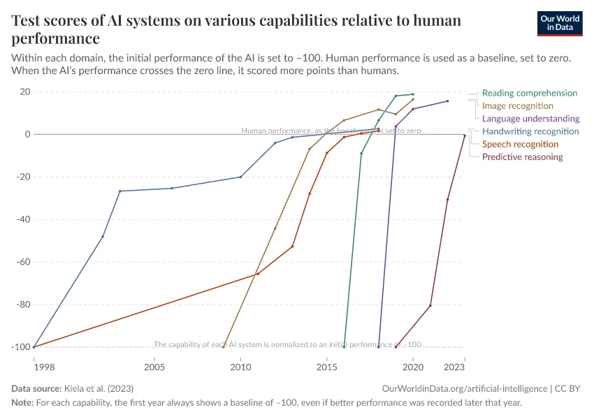
Each successive benchmark reaches human performance faster. MNIST took decades, ImageNet took years, recent language benchmarks saturate within one or two model generations (Kiela et al., “Dynabench”, NAACL 2021; Kiela, “Plotting Progress in AI”, 2023).

• SWE-bench Verified: 4% (2023) → about 90% (2026).
• GPQA Diamond: above 90%, past the PhD-expert baseline of ~65%.

Slide 29: benchmark scores relative to human performance (the zero line). Source: Our World in Data.

Warning

This makes benchmarks a poor long-term ruler: built to be hard, they stop measuring once solved.

Expert Forecasters Are Surprised by Progress

Slide 30

The Existential Risk Persuasion Tournament (XPT, 2022) ran before ChatGPT. Superforecasters were the AI skeptics, expecting the same disappointments as past AI hype. The near-term questions have since resolved (Forecasting Research Institute, “Assessing Near-Term Accuracy in the XPT”, 2025):

Benchmark (by mid-2024/25)	Experts said	Supers said	Happened
MATH high score	21%	9%	88%
MMLU high score	25%	7%	89%
IMO gold medal by 2025	9%	2%	yes, Jul 2025

The numbers are the probabilities each group placed on outcomes that then occurred, so both groups were far too pessimistic, superforecasters more so (see also Steinhardt, “AI Forecasting: One Year In”, 2022).

The GPT Series as a Compute Ladder

Slide 31

Model	Released	Params	Training compute (Epoch est., FLOP)	Note
GPT-1	Jun 2018	117M	~2 × 10¹⁹	BooksCorpus
GPT-2	Feb 2019	1.5B	~1.5 × 10²¹	staged release
GPT-3	May 2020	175B	3.1 × 10²³	in-context learning
GPT-4	Mar 2023	undisclosed	~2.1 × 10²⁵	param count is leak-only
o1	Sep 2024	n/a	n/a	first test-time-scaling model
GPT-4.5	Feb 2025	n/a	> 10²⁶	largest OpenAI pretraining run
GPT-5	Aug 2025	n/a	~5 × 10²⁵	n/a
GPT-5.5	Apr 2026	n/a	n/a	n/a
GPT-5.6 (Sol / Terra / Luna)	Jul 2026	n/a	n/a	Sol is the flagship tier (OpenAI, 9 Jul 2026)

Five orders of magnitude of training compute from GPT-1 to GPT-4 in five years (Epoch AI, model database; post-GPT-5 figures are provisional). Compare Lecture 2 on training compute.

METR: The Length of Task a Model Can Do

Slide 32

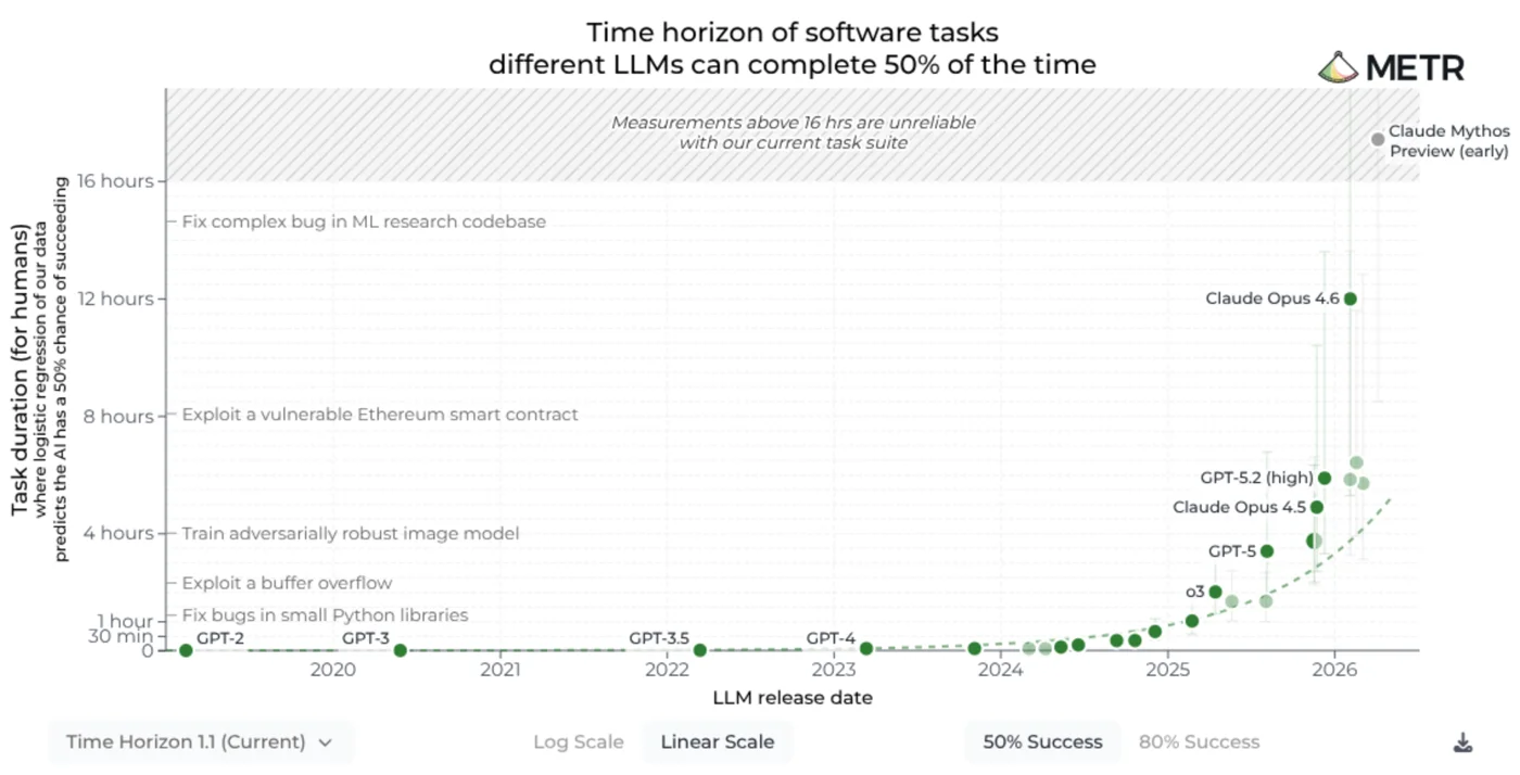
METR measures capability in a unit that extrapolates: how long a task takes a human professional (Kwa et al., “Measuring AI Ability to Complete Long Tasks”, METR 2025; METR, “Time Horizon 1.1”, Jan 2026).

• 2019-2025: doubling about every 7 months.
• Since 2023: about every 4 months.
• Frontier now: 12 to 17 hours at 50% success (Opus 4.6, Mythos).
• At a 4-month doubling, week-long and month-long tasks fall in 2026 to 2028.

Measurement caveat

Above 16 hours the measurement is unreliable (too few long tasks in the suite). See METR Time Horizon.

Slide 32 (left): time horizon on a linear axis. Source: METR.

Slide 32 (right): the same data on a log axis: a straight line, i.e. exponential growth. Source: METR.

The Horizon Depends on the Domain

Slide 33

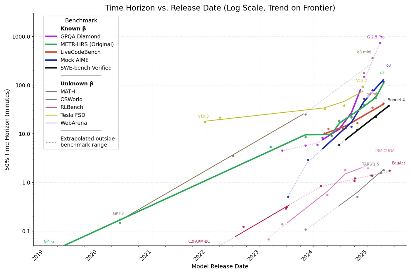
The headline curve is measured on software and reasoning tasks. Other domains sit far behind (METR, “How Does Time Horizon Vary Across Domains?”, 2025):

• Agentic GUI use (OSWorld, WebArena): horizons ~40 to 100× shorter, roughly two years behind.
• Self-driving: a ~20-month doubling, much slower.

Slide 33: time horizon by domain. Software and reasoning lead; computer use and driving lag (Moravec again). Source: METR, 2025.

Part IV: Forecasting AI Progress

Slide 34

How do people forecast AI progress based on these mechanisms?

The Classical Singularity

Slide 35

Every generation of AI researchers has extrapolated the compute curve of its day towards a hard takeoff:

Year	Who	Forecast	Status
1965	I. J. Good	”intelligence explosion”; ultraintelligent machine “within the 20th century”	miss
1988-99	Moravec	human-level compute in the 2020s-2040s	pending
1993	Vinge	superhuman AI “before 2030”	pending
1996	Yudkowsky	singularity ~2021/2025 (later repudiated, 2008)	miss
2005	Kurzweil	Turing test 2029, singularity 2045	pending

Compute-anchored forecasts (Moravec, Kurzweil) have aged best, and are not yet resolved.

Nick Land, “Meltdown” (1994)

Slide 36

Nick Land, CCRU, University of Warwick

“The story goes like this: Earth is captured by a technocapital singularity as renaissance rationalization and oceanic navigation lock into commoditization take-off. […] Nothing human makes it out of the near-future.”

(Land, “Meltdown”, 1994, in Fanged Noumena, 2011.) This is accelerationism: the same 1990s compute extrapolation as Vinge and Moravec, with the valence inverted. The singularity is something technocapital does to humanity, and in Land’s framing, welcomed.

Key point

Forecasts are never separable from culture. The same curves may support optimism, doom and acceleration depending on the subculture.

Conceptions of the Future

Slide 37

Underneath a disagreement about dates is usually a disagreement about whether the outcome is wanted. The same curve is a promise to one camp and a countdown to another. From “restrain AI to protect humanity” to “embrace what comes after”:

Position	View
Human primacy	human consciousness is a “precious flicker of light” not to be risked. Larry Page reportedly called Musk a “speciesist” for it; Musk: “I am pro-human.” (Isaacson, “Elon Musk”, 2023)
Careful transition	the rationalist and EA position: advanced AI is a real extinction risk, so making it safe should be “a global priority alongside pandemics and nuclear war” (CAIS, “Statement on AI Risk”, 2023)
Accelerationism (e/acc)	lean into the “thermodynamic bias towards futures with greater and smarter civilizations”; the direct descendant of Land’s technocapital (Jezos, “e/acc principles”, 2022)
Succession	Rich Sutton: “succession to AI is inevitable” and need not be feared: “We should not resist succession, but embrace and prepare for it.” The transhumanist “mind children” lineage from Moravec (Sutton, “AI Succession”, WAIC 2023)

These are not fringe: the people building and forecasting frontier AI hold all four views. A timeline is never only a timeline.

Concrete Forecast: Bio-Anchors

Slide 38

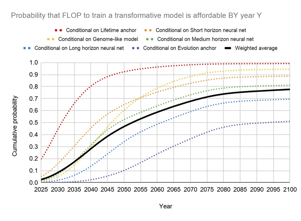
Ajeya Cotra’s 2020 report anchored the compute needed for transformative AI to biology (the human brain, evolution, a lifetime of learning), combining six estimates of required compute into a probability by year. Median: about 2050.

• 2022 update: median moved to about 2040, 15% by 2030.
• The framework fits spending and hardware trends, but assumed ~30%/year algorithmic progress. Correcting that input gives about 2030 from the same model (Alexander, “What Happened With Bio Anchors”, 2026).

Slide 38: Cotra's aggregate probability of transformative AI by year, built from six compute estimates.

Concrete Forecast: Situational Awareness

Slide 39

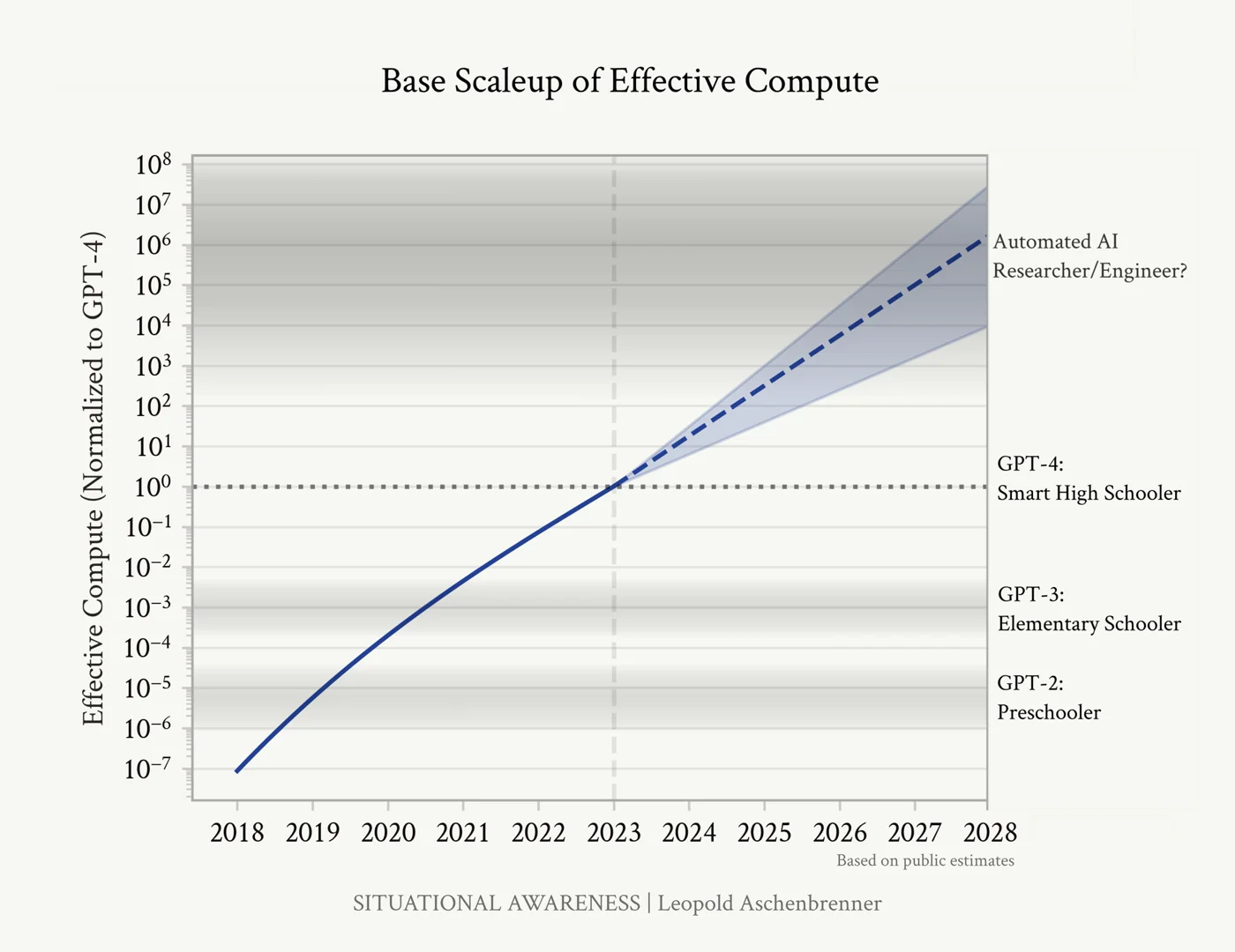
Aschenbrenner, “Situational Awareness: The Decade Ahead”, June 2024: an orders-of-magnitude (OOM) analysis of effective compute:

$$\underset{\text{physical compute}}{\underbrace{\sim 0.5\text{OOM/yr}}}+\underset{\text{algorithmic efficiency}}{\underbrace{\sim 0.5\text{OOM/yr}}}+\text{unhobbling}$$

It sums to another GPT-2-to-GPT-4 jump by 2027, then a “drop-in remote worker”, then an intelligence explosion (an “automated AI researcher” by 2027).

One-year scorecard: the straight-line infrastructure, capex and efficiency claims broadly held. The qualitative-leap and remote-worker claims did not, yet. Revenue came in near $60B against a predicted $100B.

Slide 39: effective compute, decomposed and extrapolated towards an "automated AI researcher" by 2027. Source: Aschenbrenner, 2024.

Concrete Forecast: AI 2027, the Takeoff Model

Slide 40

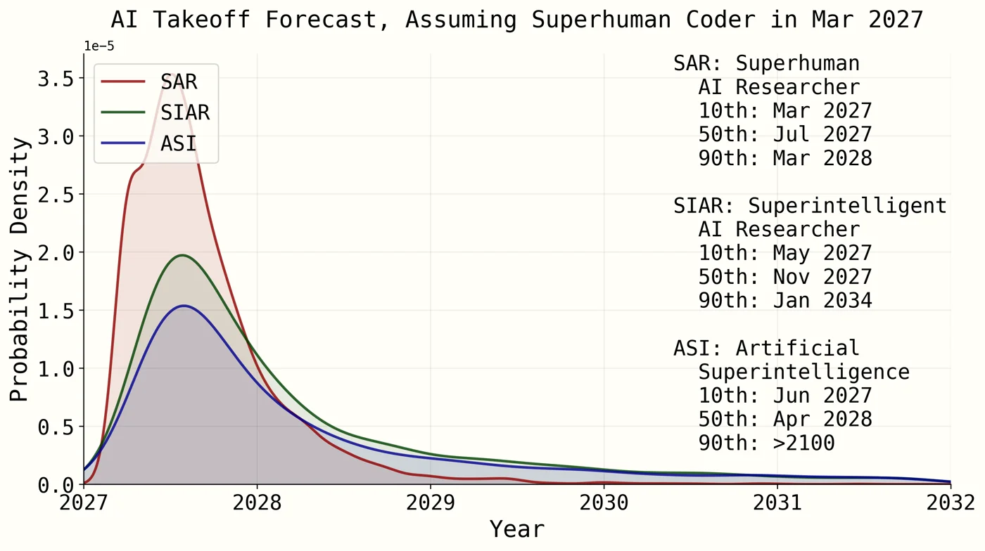
Kokotajlo, Alexander, Larsen, Lifland & Dean, “AI 2027”, April 2025: a detailed month-by-month scenario built on an explicit takeoff model. A milestone ladder, each stage with a larger AI R&D speedup multiplier:

Milestone	R&D multiplier
Superhuman Coder	~5×
Superhuman AI Researcher	~25×
Superintelligent Researcher	~250×
ASI	~2000×

Median coder-to-ASI is about one year, assuming a software-only takeoff (so Amdahl’s physical bottlenecks don’t bind). The scenario has two endings, a race and a slowdown.

Slide 40: the AI 2027 milestone ladder. Source: Kokotajlo et al., 2025.

The AI Futures Model

Slide 41

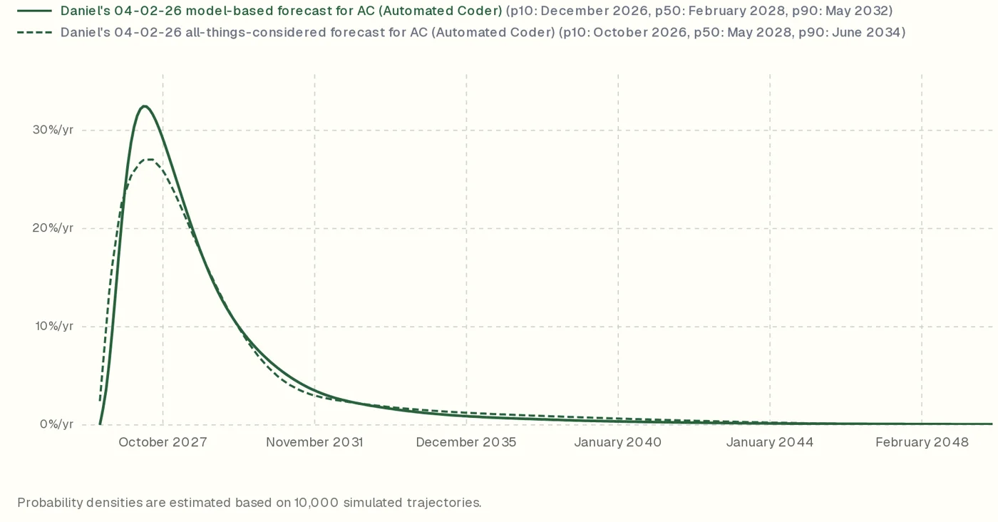
A Monte Carlo model of AI 2027 with adjustable inputs: time-horizon shape, compute and labor growth, research taste, and how fast ideas get harder to find (aifuturesmodel.com). The rebuilt model finds timelines 3 to 5 years longer than the original AI 2027 code. Different reasonable inputs give medians from the late 2020s to the mid-2030s.

Forecaster	Automated-coder median
Kokotajlo (Apr 2026)	mid-2028
Lifland (Apr 2026)	mid-2030

Slide 41: Kokotajlo's April 2026 preset. Automated-coder median: model-based February 2028, all-things-considered May 2028 ("Q1 2026 Timelines Update"). A model is a living object, not a single date.

Concrete Forecast: Europe 2031

Slide 42

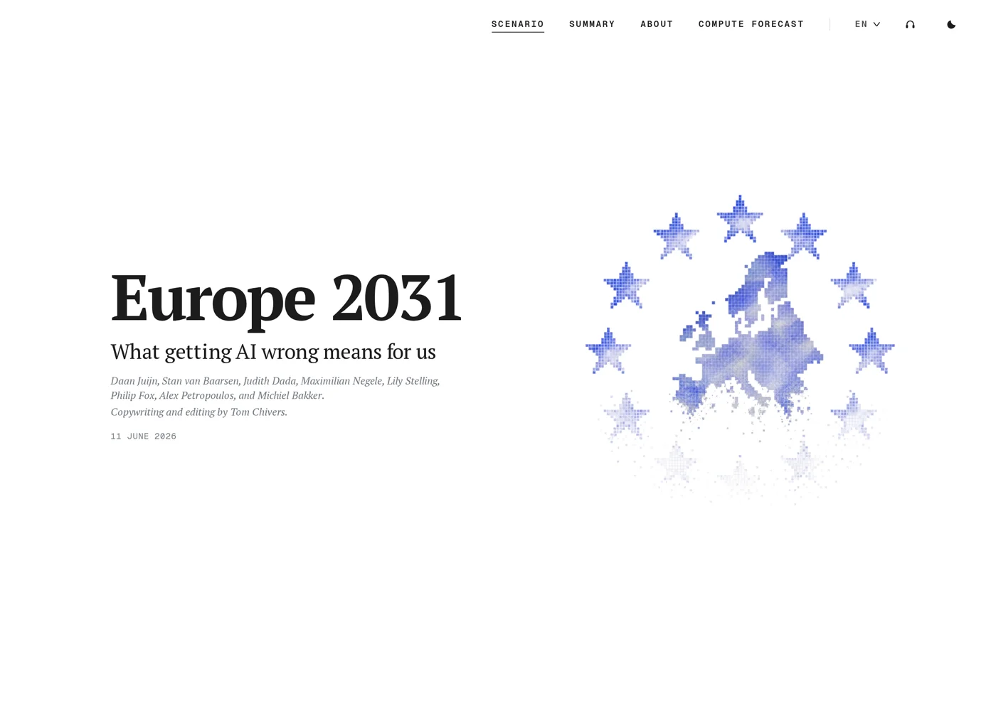
Juijn et al., “Europe 2031”, June 2026: the counterpart to AI 2027, written from and for Europe, forecasting European irrelevance by 2031.

• Europe holds about 5% of world AI compute against the US at ~80%.
• A 2029 turn to country-tiered inference rationing leaves most of Europe in a lower tier, and GDP diverges.
• ASML becomes the one card Europe holds in the endgame.

Three stated 2025 misjudgements: Europe underestimated the speed of progress, underestimated its scope, and overestimated its ability to catch up.

Slide 42: the Europe 2031 scenario.

AI 2040: Plan A

Slide 43

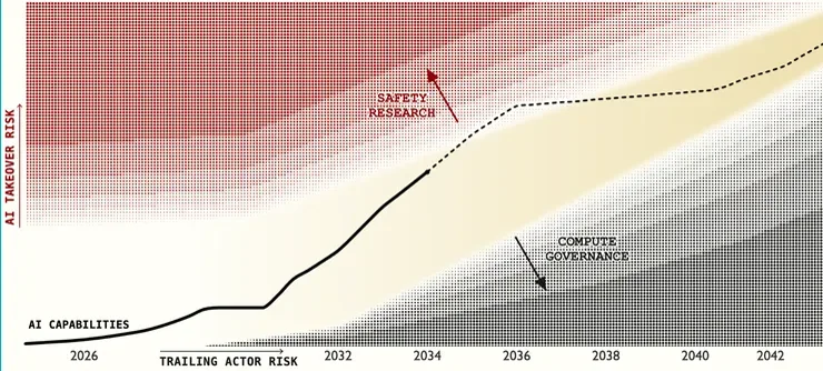
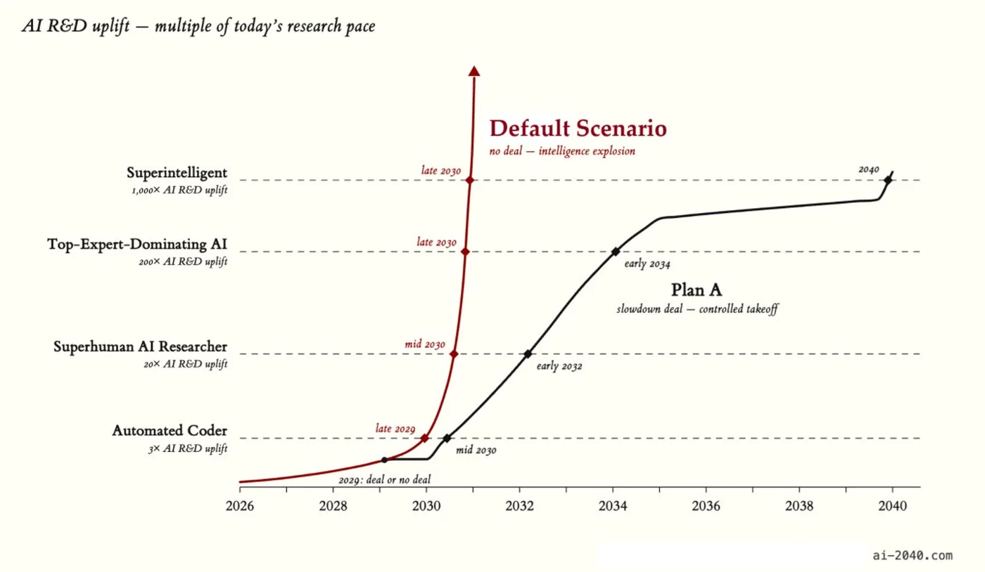
Larsen, Dean, Halstead, Lifland, Greenblatt & Kokotajlo, “AI 2040: Plan A”, 9 July 2026, by the AI 2027 team. Explicitly a recommendation, not a prediction: the same authors’ positive vision of what should happen instead.

• US-China research transparency, chip tracking, audited compute sites.
• A deliberate pause of roughly ten years (2035-2040) before a supervised intelligence explosion.
• The counterfactual no-deal superintelligence date is 2030.

Plan taxonomy: A cooperate · B fight China · C burn the lead · D race to ASI · S shut it down. Plan A is the authors’ “least bad plan we currently know of”.

Slide 43: the safe corridor, where capability rises while safety research and compute governance keep pace.

Slide 43: the milestone view, no-deal explosion vs. Plan A's controlled takeoff.

No Brakes from Here?

Slide 44

Physics allows about 2 × 10²⁹ FLOP by 2030. Whether that happens depends on six factors (Epoch AI, “The Future of AI”):

#	Factor	Why it could bind
1	Capital	the bubble question; could fail soonest if revenue lags the ~$700B/yr of capex
2	Power	Epoch’s first physical binder: grid, permitting, gigawatt-scale sites
3	Chips	packaging and memory were already the 2025 bottleneck; TSMC and ASML throughput
4	Geopolitics	Taiwan as a tail risk; export controls fragmenting the supply chain
5	Data and latency	the softest constraints before 2030; they bend the shape, not the trend
6	The physical world	robotics and biology lag regardless

The forecast for AI progress depends on how these subfactors are estimated.

Key Takeaways

Slide 45

1. Forecasting is measurable, and hard: calibration and proper scoring make forecasting a skill. Yet experts, superforecasters and markets all underpredicted 2023-2025 AI, and disagree sharply on ten-year questions.
2. The curves are real: a capability-revenue-compute flywheel, plus a second exponential in algorithms, drives compute at 4-5×/year. Scaling laws and METR horizons extrapolate strikingly straight.
3. The ceiling is physical, the timing is bottlenecked: power, chips, ASML, data and capital set the ceiling. Moravec and Amdahl set the order and the bottlenecks.
4. The scenarios are where it combines: Situational Awareness, AI 2027, the AI Futures Model and AI 2040 join the threads. Their authors’ public revisions are the best available model of current forecasting (but potentially culturally biased).

Self-Test

Question cards (14)

What is the difference between calibration and sharpness, and what is the goal of forecasting?

Answer

Calibration: among all events given probability p, a fraction p occurs. Sharpness: how concentrated (confident) the forecasts are. The goal is to maximize sharpness subject to calibration; always predicting the base rate is calibrated but useless.

What is the Brier score, and what does Murphy's decomposition say?

Answer

The mean squared error between forecast probabilities and 0/1 outcomes, $\frac{1}{N}\sum (f_i-o_i{)}^2$. It decomposes into reliability (calibration gap, want small) minus resolution (discrimination, want large) plus uncertainty (base-rate entropy, fixed by the events).

What makes a scoring rule strictly proper?

Answer

The expected score is optimized only by reporting your true belief, so there is no incentive to shade forecasts. The log score $-\log p(\text{outcome})$ is strictly proper.

Describe the forecaster's toolkit using the 40-hour-horizon example.

Answer

Decompose the question into estimable pieces: the base rate (frontier ~15 h at 50%), the reference class (doubling every ~4 to 7 months), and inside-view adjustments (data, capital, measurement noise above 16 h). Recombine into one calibrated number (55 to 70% Yes). Train calibration by logging and scoring predictions.

Why are prediction markets unreliable for long-horizon AI questions?

Answer

Capital locked into a multi-year contract forgoes market returns, which creates a no-trade region and makes long-shot dates unreliable. Markets are well calibrated over two weeks but biased over fifteen years.

What are scaling laws, and why do they make progress forecastable?

Answer

Loss falls as a power law in compute, data and parameters (Kaplan et al.), over seven orders of magnitude, and similar power laws hold across domains (Hestness et al.). A straight line on a log-log plot can be extrapolated to predict the loss of larger runs.

How do compute growth, Moore's law and algorithmic progress compare?

Answer

Moore’s law doubles transistor density about every two years; frontier training compute grows 4-5×/year, mostly from more chips and spending. Algorithms reduce compute for fixed performance ~3×/year (halving ~8 months). Together roughly 15×/year effective compute; over 2012-2023 compute contributed more, but both compound.

What are test-time compute scaling, unhobbling and overhangs, and why do they matter for forecasts?

Answer

Test-time compute: accuracy rises with inference compute (o1 AIME 83% vs. GPT-4o 12%), a second axis that later converges to the base trend. Unhobbling (RLHF, CoT, tools, scaffolds) makes existing models usable; overhangs are latent capability unlocked later by new methods. Both cause step changes that straight-line extrapolation undershoots.

What constrains scaling to 2030?

Answer

Epoch estimates ~2×10²⁹ FLOP (~5,000× GPT-4) is feasible, bounded by power (GW sites, grid, transformers), chips (TSMC concentration, CoWoS and HBM sold out, ASML’s ~60 EUV machines a year), geopolitics (Taiwan, export controls), data and latency, and above all capital: if revenue lags ~$700B/yr capex, the flywheel stalls first.

What do Moravec's paradox and Amdahl's law imply for AI progress?

Answer

Moravec: abstract reasoning is easy for machines but perception and mobility are hard, so robotics and physical domains lag. Amdahl: with serial fraction s, speedup ≤ 1/s, so automating 90% of research caps speedup at 10×. Whether this binds AI R&D is disputed (METR yes; AI 2027 and Epoch GATE argue better experiment selection or capital break it).

Why are benchmarks a poor long-term ruler, and how did forecasters do?

Answer

Benchmarks saturate ever faster (SWE-bench Verified 4% → ~90%), so they stop measuring once solved. In the 2022 XPT, experts and superforecasters gave low probabilities (e.g. MATH 21%/9%, IMO gold 9%/2%) to outcomes that happened; superforecasters were the most skeptical.

What does the METR time horizon measure and show, and what are its limits?

Answer

The length of tasks (in human professional time) a model completes with 50% success. It doubled about every 7 months (2019-2025), about every 4 months since 2023, frontier at 12 to 17 h. Limits: unreliable above 16 h, and domain-dependent: GUI agents are 40-100× shorter, self-driving doubles every ~20 months.

Compare Bio-Anchors, Situational Awareness and AI 2027.

Answer

Bio-Anchors anchors required compute to biology; median ~2050, updated to ~2040, and ~2030 with corrected algorithmic progress. Situational Awareness adds ~0.5 OOM/yr compute and ~0.5 OOM/yr algorithms plus unhobbling, predicting an automated AI researcher by 2027 (infrastructure claims held, qualitative leaps not yet). AI 2027 models a software-only takeoff with R&D multipliers from ~5× to ~2000× and coder-to-ASI in about a year; the AI Futures Model rebuild gives 3 to 5 years longer timelines.

Why is "a timeline never only a timeline"?

Answer

Disagreements about dates usually hide disagreements about whether the outcome is wanted: human primacy, careful transition, accelerationism and succession read the same curves as a threat, a risk to manage, a promise or an inevitability. Forecasts are embedded in subcultures, so their authors’ revisions are informative but potentially biased.

Multiple Choice

Multiple choice (5)

A forecaster always predicts the base rate of 30% for rain. Which is true?

• The forecasts are calibrated but not sharp.

• The forecasts are sharp but not calibrated.

• The Brier score is minimal.

• The resolution term of the Brier score is large.

Explanation

It rains 30% of the time when 30% is said, so calibrated, but the forecasts never discriminate between days: zero sharpness and zero resolution.

Roughly how fast does frontier AI training compute grow per year?

• 1.4× (Moore’s law)

• 2×

• 4-5×

• 100×

Explanation

Epoch AI: 4-5× per year, roughly an order of magnitude faster in exponent than Moore’s law; algorithms add ~3× on top.

If 90% of AI research is automated with infinite speedup and 10% stays serial, what is the maximum overall speedup by Amdahl's law?

• 90×

• 10×

• 1.9×

• unbounded

Explanation

speedup ≤ 1/s = 1/0.1 = 10.

Which statements about the METR time horizon are true? (Select all that apply.)

• It measures task length in human professional time at 50% success.

• It has doubled roughly every 4 months since 2023.

• It is equally fast in all domains, including self-driving.

• Measurements above ~16 hours are unreliable.

Explanation

Other domains lag: GUI use is 40-100× shorter and self-driving doubles only every ~20 months.

What was the main correction to Cotra's Bio-Anchors model that pulls its median to ~2030?

• a higher estimate of brain compute

• faster algorithmic progress than the assumed ~30% per year

• slower hardware progress

• ignoring spending growth

Explanation

Algorithmic efficiency grows ~3× per year, far more than the 30% per year assumed in 2020.

References

All sources cited on the slides, in slide order (69 entries)

Slide	Source	Key point
5	Dawid, “The Well-Calibrated Bayesian”, JASA 1982	calibration
5	Gneiting, Balabdaoui & Raftery, JRSS-B 2007	sharpness subject to calibration
6	Murphy, “A New Vector Partition of the Probability Score”, 1973	Brier decomposition
6	Gneiting & Raftery, “Strictly Proper Scoring Rules”, JASA 2007	proper scoring
6	calibration.city	market calibration data
7	Fatebook, Calibration, Pastcasting, Sage	calibration training
7	LessWrong, “Forecasting & Prediction”	forecasting background
8	Yudkowsky, “Making Beliefs Pay Rent”, 2007	falsifiable beliefs
9	Wolfers & Zitzewitz, “Prediction Markets”, JEP 2004	prediction markets
9	”Can Interest-Bearing Positions Solve the Long-Horizon Problem in Prediction Markets?”, 2026	long-horizon bias
10	Goel et al., “FutureSim”, 2026	AI as forecaster
10	Forecasting Research Institute	forecasting research
12	Hestness et al., 2017	power-law scaling
12	Kaplan et al., “Scaling Laws for Neural Language Models”, 2020	LLM scaling laws
13	Our World in Data, “Moore’s Law”	transistor density
13	Epoch AI, “Training compute grows by 4-5x per year”	compute trend
14	Ho et al., “Algorithmic Progress in Language Models”, 2024	~3×/year algorithms
14	Erdil & Besiroglu, “Algorithmic Progress in Computer Vision”, 2022	vision
14	Epoch AI Trends	trend data
15	OpenAI, “Learning to Reason with LLMs”, 2024	test-time compute
15	Muennighoff et al., “s1: Simple Test-Time Scaling”, 2025	test-time scaling
15	Epoch, “How far can reasoning models scale?“	reasoning compute trend
16, 39	Aschenbrenner, “Situational Awareness”, 2024	unhobbling, effective compute
17	Our World in Data, “Economic Growth”	world GDP
18	Sevilla et al., “Can AI Scaling Continue Through 2030?”, 2024	2030 constraints
19	Epoch AI, Frontier Data Centers Hub	GW sites
19	Epoch, “Power demands of frontier AI training”	power
20	Epoch AI, “AI chip supply chain constraints”	CoWoS, HBM
20	CSIS, “Taiwan’s Semiconductor Dominance”	TSMC
21	ASML Q4 2025 results	EUV shipments
22	Sutton, “The Bitter Lesson”, 2019	general methods scale
23	Epoch AI, Anthropic vs. OpenAI revenue	revenue
23	Epoch, “How well did forecasters predict 2025 AI progress?“	revenue underestimated
24	Moravec, “Mind Children”, 1988	Moravec’s paradox
25	”Limits to biomedical research acceleration through general-purpose AI”, Sci. Reports 2025	biology latency
25	Narayanan & Kapoor, “AI as Normal Technology”, 2025	diffusion view
26	Amdahl, 1967	Amdahl’s law
26	METR, “A simpler AI timelines model”, 2026	strict Amdahl
26	AI 2027 Takeoff Forecast	takeoff model
26	Epoch GATE	capital accumulation
29	Kiela et al., “Dynabench”, NAACL 2021	benchmark saturation
29	Kiela, “Plotting Progress in AI”, 2023	benchmark saturation
29	Our World in Data, test scores relative to humans	chart data
30	FRI, “Assessing Near-Term Accuracy in the XPT”, 2025	forecasters surprised
30	Steinhardt, “AI Forecasting: One Year In”, 2022	forecasts undershoot
31	Epoch AI, model database	GPT compute ladder
31	OpenAI, GPT-5.6, 2026	newest model
32	Kwa et al., “Measuring AI Ability to Complete Long Tasks”, METR 2025	time horizon
32	METR, “Time Horizon 1.1”, 2026	updated horizons
33	METR, “How Does Time Horizon Vary Across Domains?”, 2025	domains
35	Good, 1965	intelligence explosion
35	Vinge, 1993	singularity
35	Moravec, 1998	human-level compute
35	Kurzweil, 2001	accelerating returns
35	Yudkowsky’s later reckoning, 2008	repudiated forecast
36	Land, “Meltdown”, 1994	accelerationism
37	Isaacson, “Elon Musk”, 2023	human primacy
37	CAIS, “Statement on AI Risk”, 2023	careful transition
37	Jezos, “e/acc principles”, 2022	accelerationism
37	Sutton, “AI Succession”, WAIC 2023	succession
38	Cotra, “Biological Anchors”, 2020	bio anchors
38	Cotra, 2022 update	median ~2040
38	Alexander, “What Happened With Bio Anchors”, 2026	retrospective
40	Kokotajlo et al., “AI 2027”, 2025	takeoff scenario
41	aifuturesmodel.com	AI Futures Model
41	”Q1 2026 Timelines Update”, 2026	revised medians
42	Juijn et al., “Europe 2031”, 2026	European scenario
43	Larsen et al., “AI 2040: Plan A”, 2026	recommended plan
44	Epoch AI, “The Future of AI”	constraints overview

Related

• Previous: Lecture 12: Automating AI R&D · Course: Overview
• Exam and reference: Exam Structure · Study Plan · Formula Sheet · Glossary
• Concepts: Forecasting and Calibration, Scaling Laws, METR Time Horizon, Training Compute, Recursive Self-Improvement
• First look at METR time horizons: Lecture 1.