Lecture 4: Algorithmic Stability

TL;DR

1. Stability principle: if the output of an algorithm changes only a little when one training point is replaced, the algorithm generalizes. Unlike capacity bounds, this looks at the actual algorithm, not the whole function class.
2. $S_n^i$ is $S_n$ with the $i$-th point replaced by an independent $Z_i^{\prime }$. Average stability ${\Delta }_{av}(A,n)$ averages the loss change on the replaced point; uniform stability ${\Delta }_{\sup }(A,n)={\sup }_{i,S_n,S_n^i,Z}|\ell (f(S_n),Z)-\ell (f(S_n^i),Z)|$. Always ${\Delta }_{av}\le {\Delta }_{\sup }$.
3. Proposition 1: $E(R(f(S_n))-R_{S_n}(f(S_n)))={\Delta }_{av}(A,n)$: the expected generalization gap equals the average stability.
4. Theorem 2: with loss bounded by $M$ and ${\beta }_n={\Delta }_{\sup }(A,n)$, with probability $1-\delta$: $R(f(S_n))\le R_{S_n}(f(S_n))+{\beta }_n+(2n{\beta }_n+M)\sqrt{\log (1/\delta )/(2n)}$. The gap vanishes iff ${\beta }_n=o(1/\sqrt{n})$.
5. Stability alone does not give consistency (a constant predictor is perfectly stable); stability plus (approximate) ERM does.
6. Theorem 3: ERM with a $\mu$-strongly convex, $L$-Lipschitz loss is uniformly stable with ${\Delta }_{\sup }\le 4L^2/(\mu n)$, independent of the complexity of $\mathcal{F}$. Theorems 4-6: GD and SGD on convex, $\beta$-smooth, $L$-Lipschitz losses with step sizes ${\eta }_t<2/\beta$ have ${\Delta }_{\sup }\le \frac{2L^2}{n}{\sum }_{t=1}^T{\eta }_t$ (non-convex: $\approx T^{1-1/(\beta c+1)}/n$): fewer steps, more stable.

Exam relevance

• Real exam, task type “algorithmic stability” (4 P): the bound of Theorem 2 is given together with a table of candidate rates $B_n$ ($1/n$, $1/\sqrt{n}$, …); tick yes/no whether the bound goes to 0. Key fact: it vanishes iff $\sqrt{n}{B}_n\to 0$. See the task and the widget.
• Mock exam, task 6: uniform stability of the averaging rule with the squared loss, then what it implies (Proposition 1). Train it with the own-number version.
• Multiple choice: ${\Delta }_{av}$ vs. ${\Delta }_{\sup }$, stability vs. consistency, the assumptions of Theorem 3, why the plain squared loss is not strongly convex.
• Sheet 5: 1-NN is not uniformly stable at rate $1/n$ but is stable on average; the averaging algorithm has $\beta \le 2/n$; stability of one-pass SGD.

Overview: 1. Motivation and definitions, 2. Stability implies generalization, 3. ERM with strongly convex loss is stable, 4. (S)GD on smooth losses is stable.

Motivation and key definitions

Why stability?

Slides 3-6

(Literature: Hardt and Recht Sec. 6.4, Mohri Sec. 11.2, Shalev-Shwartz and Ben-David Sec. 13.2. Key original references: Bousquet and Elisseeff 2002 for the standard bound; Shalev-Shwartz, Shamir, Srebro and Sridharan 2010 for “stability is sufficient and necessary for learning”; Hardt, Recht and Singer 2016 for the stability of SGD.)

Motivation 1. The standard approach of SLT proves generalization by bounding the capacity of the function class. This is often technically challenging and gives worst-case guarantees over all functions in the class instead of looking at the actual optimizers. In the perceptron bound (Lecture 2) we already saw the stability principle: if the result of a learning algorithm changes only a little when we fiddle with the data a little, the algorithm tends to generalize well.

Motivation 2. The LLN or the CLT hold as long as no single data point has much more influence than the others: the influence of one $X_i$ on the empirical average $\frac{1}{n}{\sum }_i{X}_i$ is “of the order $1/n$“. Stability measures, in the same spirit, the influence of single data points on the empirical risk.

Definitions

Slides 7-10

Samples and notation

Two samples drawn i.i.d. from $P$: $S_n=\{(X_1,Y_1),\dots ,(X_n,Y_n)\}$ and $S_n^{\prime }=\{(X_1^{\prime },Y_1^{\prime }),\dots ,(X_n^{\prime },Y_n^{\prime })\}$. The adapted sample $S_n^i$ replaces the $i$-th point of $S_n$ by the $i$-th point of $S_n^{\prime }$:

$$S_n^i:=\{(X_1,Y_1),\dots ,(X_{i-1},Y_{i-1}),(X_i^{\prime },Y_i^{\prime }),(X_{i+1},Y_{i+1}),\dots ,(X_n,Y_n)\}$$

Shorthand: $Z_i=(X_i,Y_i)$ and $\ell (f,Z):=\ell (f(X),Y)$. $A(S_n)$ or $f(S_n)$ is the function learned by algorithm $A$ on $S_n$, and $R_{S_n}(f)=\frac{1}{n}{\sum }_{i=1}^n\ell (f(X_i),Y_i)$ the empirical risk on $S_n$ (analogously $R_{S_n^{\prime }}$, $R_{S_n^i}$).

Average stability

$${\Delta }_{av}(A,n):=E_{S_n,S_n^{\prime }}\left(\frac{1}{n}\sum _{i=1}^n\ell (f(S_n),Z_i^{\prime })-\ell (f(S_n^i),Z_i^{\prime })\right)$$

For each $i$ we compare $f(S_n)$, trained on the original sample, with $f(S_n^i)$, trained with $Z_i$ replaced by $Z_i^{\prime }$, both evaluated on $Z_i^{\prime }$. Note that $Z_i^{\prime }$ is a test point for $S_n$ but a training point for $S_n^i$.

Uniform stability

For $S_n$ and $S_n^i$ that differ in exactly one point, and a completely new test point $Z$ (independent of both samples):

$${\Delta }_{\sup }(A,n):=\underset{i=1,\dots ,n}{\sup }\underset{S_n,S_n^i}{\sup }\underset{Z}{\sup }|\ell (f(S_n),Z)-\ell (f(S_n^i),Z)|$$

Obviously ${\Delta }_{av}(A,n)\le {\Delta }_{\sup }(A,n)$.

Mini example: the averaging algorithm (Sheet 5)

Regression on $\mathcal{X}\times [0,1]$ with the squared loss, $A(S)(x)=\frac{1}{n}{\sum }_i{y}_i$ for every $x$. Replacing one label changes the prediction by $|y_i-y_i^{\prime }|/n\le 1/n$. With $\bar{y},{\bar{y}}^{\prime }$ the two predictions and a test label $y\in [0,1]$: $|(\bar{y}-y{)}^2-({\bar{y}}^{\prime }-y{)}^2|=|\bar{y}-{\bar{y}}^{\prime }|\cdot |\bar{y}+{\bar{y}}^{\prime }-2y|\le \frac{1}{n}\cdot 2$. So ${\Delta }_{\sup }\le 2/n$.

Not every algorithm is uniformly stable

1-nearest neighbour (Sheet 5): on $\mathcal{X}=\{a,b\}$, replacing the one training point at $a$ can flip the prediction at a test point near $a$, so the loss changes by 1 and ${\Delta }_{\sup }=1$, not $1/n$. On average, though, a single point is the nearest neighbour of a random test point only with probability $1/n$.

Algorithmic stability implies generalization

The expected generalization gap

Slides 11-14

(Literature: Mohri textbook.)

Proposition 1 (expected generalization gap equals average stability)

$$E(\underset{\text{true error}}{\underbrace{R(f(S_n))}}-\underset{\text{empirical error}}{\underbrace{R_{S_n}(f(S_n))}})={\Delta }_{av}(A,n)$$

with the expectation over the training sample $S_n$.

Proof

Write both expectations as averages over $n$ equal terms.

True error. Blow it up into a sum of equal terms and write out $R$ with the independent test points $z_i^{\prime }$:

$$E(R(f(S_n)))=E(\frac{1}{n}\sum _{i=1}^{n}R(f(S_n)))=E(\frac{1}{n}\sum _{i=1}^n\ell (f(S_n),z_i^{\prime }))$$

Empirical error. By definition, with $z_i$ a training point, then rename: $(S_n,z_i)$ has the same distribution as $(S_n^i,z_i^{\prime })$, so

$$E(R_{S_n}(f(S_n)))=E(\frac{1}{n}\sum _{i=1}^n\ell (f(S_n),z_i))=E(\frac{1}{n}\sum _{i=1}^n\ell (f(S_n^i),z_i^{\prime }))$$

Subtracting gives $E(\frac{1}{n}{\sum }_i\ell (f(S_n),z_i^{\prime })-\ell (f(S_n^i),z_i^{\prime }))={\Delta }_{av}(A,n)$. $\square$

Discussion

This points in an interesting direction (bounding the generalization error by stability), but average stability is hard to evaluate. The stronger notion of uniform stability is easier to bound in practice and gives a nice high-probability bound, proved with McDiarmid’s inequality (Lecture 3).

Uniformly stable algorithms generalize

Slides 15-19

Theorem 2 (generalization bound for stable algorithms)

Assume the loss is bounded by a constant $M>0$ and let ${\beta }_n:={\Delta }_{\sup }(A,n)$ be the uniform stability of $A$ on $n$ samples. Then with probability at least $1-\delta$ over the samples $S_n$:

$$R(f(S_n))\le R_{S_n}(f(S_n))+{\beta }_n+(2n{\beta }_n+M)\sqrt{\frac{\log (1/\delta )}{2n}}$$

Proof sketch (full proof: Mohri, Sec. 11.2, p. 268)

Apply McDiarmid to $\phi (S_n)=R(f(S_n))-R_{S_n}(f(S_n))$.

Step 1: bounded differences. By the triangle inequality

$$|\phi (S_n^i)-\phi (S_n)|\le \underset{(1)}{\underbrace{|R(f(S_n^i))-R(f(S_n))|}}+\underset{(2)}{\underbrace{|R_{S_n^i}(f(S_n^i))-R_{S_n}(f(S_n))|}}$$

(1): $|E(\ell (f(S_n^i),z))-E(\ell (f(S_n),z))|\le E|\ell (f(S_n^i),z)-\ell (f(S_n),z)|\le {\beta }_n$ by the definition of stability.

(2): write the empirical risks as sums and split off the term $j=i$:

$$|R_{S_n^i}(f(S_n^i))-R_{S_n}(f(S_n))|\le \frac{1}{n}\sum _{j\ne i}\underset{\le {\beta }_n}{\underbrace{|\ell (f(S_n^i),z_j)-\ell (f(S_n),z_j)|}}+\frac{1}{n}\underset{\le M}{\underbrace{|\ell (f(S_n^i),z_i^{\prime })-\ell (f(S_n),z_i)|}}\le {\beta }_n+\frac{M}{n}$$

So $|\phi (S_n^i)-\phi (S_n)|\le 2{\beta }_n+M/n=:c_i$.

Step 2: McDiarmid. With ${\sum }_i{c}_i^2=n(2{\beta }_n+M/n{)}^2$:

$$P(\phi (S)-E(\phi (S))>\epsilon )\le \exp \left(-\frac{2{\epsilon }^2}{n(2{\beta }_n+M/n{)}^2}\right)=:\delta$$

Solving for $\epsilon$: with probability at least $1-\delta$, $\phi (S)\le E(\phi (S))+(2n{\beta }_n+M)\sqrt{\log (1/\delta )/(2n)}$. Finally $E(\phi (S))={\Delta }_{av}\le {\Delta }_{\sup }={\beta }_n$ by Proposition 1. $\square$

Trap

On slide 16 the bound for term (2) reads "${\beta }_n+\mu /n$"; it should be $M/n$ (the loss bound), as on slide 18.

Discussion: which rates are good enough?

Slide 20

As soon as we can bound the uniform stability ${\beta }_n$ of an algorithm, we can plug it into Theorem 2. The key term is

$${\beta }_n+\frac{(2n{\beta }_n+M)}{\sqrt{n}}\sqrt{\log (1/\delta )}$$

and it goes to 0 if ${\beta }_n\to 0$ and $\frac{n{\beta }_n}{\sqrt{n}}\approx \sqrt{n}{\beta }_n\to 0$ as $n\to \infty$.

The condition to remember

The uniform stability ${\beta }_n$ needs to be of order $o(1/\sqrt{n})$ to be useful. ${\beta }_n=1/n$ works; ${\beta }_n=1/\sqrt{n}$ does not: then $2n{\beta }_n\sqrt{\log (1/\delta )/(2n)}=\sqrt{2\log (1/\delta )}$ stays constant.

The gap of Theorem 2 for several rates βₙ against n. Switch on quiz mode to hide the answers and decide yes/no yourself, like in the exam table. The dashed curve is your own rate n^(−α).

Task: which stability rates are good enough?

Exam-style task: stability rates (4 P)

Use Theorem 2 with $M=1$.

${\beta }_n$	bound → 0?
$1/n$
$1/\sqrt{n}$
$\log n/n$
$n^{-3/4}$
$1/\log n$
$\log n/\sqrt{n}$

(a) (1.5 P, easy) Fill in yes/no for each rate.

(b) (1 P, harder) Evaluate the gap ${\beta }_n+(2n{\beta }_n+M)\sqrt{\log (1/\delta )/(2n)}$ for ${\beta }_n=1/n$, $n=10^4$ and $\delta =0.05$.

(c) (1.5 P, transfer) GD with constant step size $\eta <2/\beta$ has ${\beta }_n\le \frac{2L^2}{n}\eta T$ after $T$ steps (Theorem 4). How may the number of steps $T=T(n)$ grow so that Theorem 2 still gives a vanishing gap?

Solution

(a) Check $\sqrt{n}{\beta }_n\to 0$: $1/n$ yes ($1/\sqrt{n}$), $1/\sqrt{n}$ no (constant 1), $\log n/n$ yes ($\log n/\sqrt{n}$), $n^{-3/4}$ yes ($n^{-1/4}$), $1/\log n$ no ($\sqrt{n}/\log n\to \infty$), $\log n/\sqrt{n}$ no ($\log n\to \infty$). (0.25 P each)

(b) ${\beta }_n=10^{-4}$, $2n{\beta }_n+M=3$, $\sqrt{\ln 20/(2\cdot 10^4)}=\sqrt{1.498\cdot 10^{-4}}\approx 0.0122$. Gap $\approx 10^{-4}+3\cdot 0.0122\approx 0.037$. (1 P)

(c) $\sqrt{n}{\beta }_n\le 2L^2\eta T/\sqrt{n}\to 0$ iff $T=o(\sqrt{n})$. For example $T=n^{1/4}$ works, $T=n$ (one step per training point) does not. More steps make GD less stable: an argument for early stopping. (1.5 P)

Stability does not immediately imply consistency

Slides 21-22

Theorem 2 only says that for the function $f(S_n)$ picked by the algorithm, $R(f(S_n))\approx R_n(f(S_n))$. We do not (yet) know whether this function is anywhere close to the best in $\mathcal{F}$, nor to the Bayes predictor.

Counterexample

A naive algorithm that always predicts 0 is perfectly stable (${\Delta }_{\sup }=0$) and satisfies $R(f(S_n))=R_n(f(S_n))$, but it is not the best in $\mathcal{F}$. For consistency we need a separate condition about the (empirical) risk of the classifier.

Stability + approximate ERM ⇒ consistency

Run ERM on a huge class $\mathcal{F}$; if the ERM solution is uniformly stable, we get consistency:

$$\begin{array}{rl}R(f_n)-R(f_{\mathcal{F}})=& \underset{\text{(1) small if ERM is stable (Theorem 2)}}{\underbrace{R(f_n)-R_n(f_n)}}\\ +& \underset{\text{(2) }\le 0\text{ since }{f}_n\text{ minimizes}}{\underbrace{R_n(f_n)-R_n(f_{\mathcal{F}})}}\\ +& \underset{\text{(3) small by the LLN for the fixed }{f}_{\mathcal{F}}}{\underbrace{R_n(f_{\mathcal{F}})-R(f_{\mathcal{F}})}}\end{array}$$

Task: stability of an averaging rule

Exam-style task: an averaging rule with the absolute loss (4 P)

Labels $y\in [0,2]$, the algorithm predicts the mean label $A(S)(x)=\frac{1}{n}{\sum }_{i=1}^n{y}_i$ for every $x$, and the loss is the absolute loss $\ell (f,(x,y))=|f(x)-y|$.

(a) (1 P, easy) Show that $A(S)$ and $A(S^i)$ differ pointwise by at most $2/n$.

(b) (1.5 P, harder) Show ${\Delta }_{\sup }(A,n)\le 2/n$ and give the loss bound $M$.

(c) (1.5 P, transfer) Evaluate the gap of Theorem 2 for $n=800$, $\delta =0.05$. What does the result say about $R(A(S))$, and what does it not say?

Solution

(a) Only the $i$-th label changes: $|A(S)(x)-A(S^i)(x)|=\frac{1}{n}|y_i-y_i^{\prime }|\le \frac{2}{n}$. (1 P)

(b) The absolute loss is 1-Lipschitz in the prediction: $||a-y|-|b-y||\le |a-b|\le 2/n$ for every test point, so ${\Delta }_{\sup }\le 2/n$. Predictions and labels lie in $[0,2]$, so $M=2$. (1.5 P)

(c) ${\beta }_n=0.0025$, $2n{\beta }_n+M=4+2=6$, $\sqrt{\ln 20/1600}\approx 0.0433$: gap $\approx 0.0025+0.26=0.26$. With probability 0.95 the true risk is at most the training risk plus $0.26$, and the gap tends to 0 because ${\beta }_n=O(1/n)$: no overfitting. It does not say that the risk is small: a constant predictor can be far from the regression function (large approximation error). (1.5 P)

ERM with strongly convex loss function is stable

Motivation and strongly convex functions

Slides 23-27

(Literature: Hardt and Recht, Chapter 6, p. 111, Theorem 4.) Machine learning often minimizes a loss on training data (ERM). For small classes we can prove uniform convergence; if the class is too large for SLT, uniform stability might help. Question: is ERM uniformly stable? Answer: only under very strong assumptions on the loss.

$\mu$-strongly convex

A differentiable $f:\mathcal{X}\to \mathbb{R}$ on a convex domain $\mathcal{X}\subset {\mathbb{R}}^d$ is $\mu$-strongly convex ($\mu >0$) if for all $x,y$

$$f(y)\ge f(x)+\nabla f(x)(y-x)+\frac{\mu }{2}\Vert y-x{\Vert }^2$$

In 1d with $f$ twice differentiable: convex iff $f^{\prime \prime }\ge 0$, strongly convex if $f^{\prime \prime }(x)>\mu$ everywhere (a lower bound $\mu$ on the curvature). In ${\mathbb{R}}^d$: the smallest eigenvalue of the Hessian is at least $\mu$.

Slide 25: f lies above the tangent plus (μ/2)‖y − x‖².

Slide 27: strongly convex (left) vs. convex with a flat part (right).

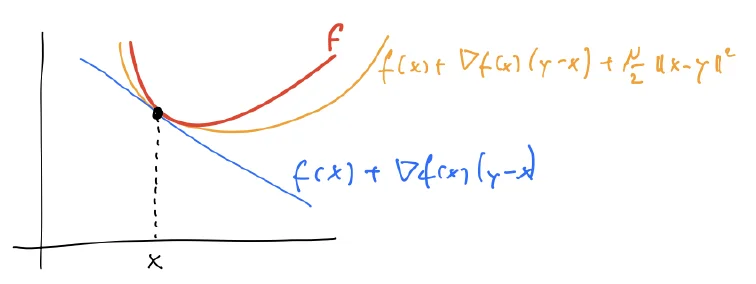
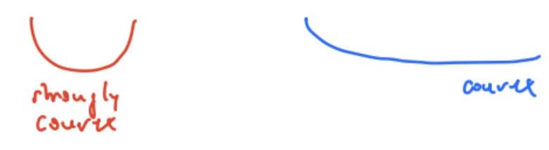
If the loss is strongly convex, the empirical risk is strongly convex with the same $\mu$. Then there always is a global optimum and it is not “hidden” in flat parts; GD and SGD easily find it.

Theorem 3: ERM is stable for strongly convex losses

Slides 28-33

Theorem 3 (ERM for strongly convex loss functions is stable)

Let each function in $\mathcal{F}$ be parameterized by $w\in {\mathbb{R}}^d$. Assume the loss $\ell (f_w(x),y)$ is $\mu$-strongly convex in $w$ and $L$-Lipschitz in $w$, for every $(x,y)$. Then the empirical risk minimizer $f_{ERM}$ is uniformly stable with

$${\Delta }_{\sup }(f_{ERM},n)\le \frac{4L^2}{\mu n}$$

First discussion

• The theorem is about the empirical risk minimizer itself, not about an algorithm that tries to find it.
• The complexity of $\mathcal{F}$ does not show up anywhere. This is great.
• ${\Delta }_{\sup }$ scales as $1/n$, so Theorem 2 gives a vanishing gap and, with the ERM argument above, consistency.
• The assumptions are really strong. Promising, but not yet a solution for more complex losses.

Proof of Theorem 3

Fix $S=(z_1,\dots ,z_i,\dots ,z_n)$, $S^{\prime }=(z_1,\dots ,z_i^{\prime },\dots ,z_n)$ and a test point $z$. Let $w_S$, $w_{S^{\prime }}$ be the ERM minimizers. Because $\ell$ is $L$-Lipschitz, $|\ell (w_S,z)-\ell (w_{S^{\prime }},z)|\le L\Vert w_S-w_{S^{\prime }}\Vert$, so it suffices to show $\Vert w_S-w_{S^{\prime }}\Vert \le \frac{4L}{\mu n}$.

Step 1. A $\mu$-strongly convex $g$ with minimizer $w^{\ast }$ satisfies $\frac{\mu }{2}\Vert w-w^{\ast }{\Vert }^2\le g(w)-g(w^{\ast })$ (definition plus $\nabla g(w^{\ast })=0$). The empirical risk $R_S$ is $\mu$-strongly convex with minimizer $w_S$, so

$$\frac{\mu }{2}\Vert w_{S^{\prime }}-w_S{\Vert }^2\le R_S(w_{S^{\prime }})-R_S(w_S)$$

Step 2. Write $R_S$ as a sum, split off the term $i$, add and subtract the terms with $z_i^{\prime }$ and use that $w_{S^{\prime }}$ minimizes $R_{S^{\prime }}$:

$$\begin{array}{rl}{R}_S(w_{S^{\prime }})-R_S(w_S)& =\frac{1}{n}(\ell (w_{S^{\prime }},z_i)-\ell (w_S,z_i))+\frac{1}{n}(\ell (w_S,z_i^{\prime })-\ell (w_{S^{\prime }},z_i^{\prime }))+\underset{\le 0}{\underbrace{(R_{S^{\prime }}(w_{S^{\prime }})-R_{S^{\prime }}(w_S))}}\\ & \le \frac{2L}{n}\Vert w_{S^{\prime }}-w_S\Vert \text{(Lipschitz twice)}\end{array}$$

Step 3. Combine: $\frac{\mu }{2}\Vert w_S-w_{S^{\prime }}{\Vert }^2\le \frac{2L}{n}\Vert w_S-w_{S^{\prime }}\Vert$, so $\Vert w_S-w_{S^{\prime }}\Vert \le \frac{4L}{\mu n}$ and ${\Delta }_{\sup }\le L\cdot \frac{4L}{\mu n}=\frac{4L^2}{\mu n}$. $\square$

Two small slips on the slides

Slide 31 writes $R_S(w_S)-R_S(w_{S^{\prime }})$ on the right of step 1; since $w_S$ minimizes $R_S$, the non-negative difference is $R_S(w_{S^{\prime }})-R_S(w_S)$. Slide 33 ends with ${\Delta }_{\sup }\le 4L/(\mu n)$; the Lipschitz step adds a factor $L$, giving $4L^2/(\mu n)$ as in the theorem.

Discussing the assumption

Slide 34

The squared loss of a linear model is not strongly convex

$\ell (w,(x,y))=(⟨w,x⟩-y{)}^2$ has gradient $2(⟨w,x⟩-y)x$ and Hessian $2x{x}^{\top }$. The Hessian has rank 1, so its smallest eigenvalue is 0 (for $d>1$): not strongly convex. Adding regularization $\lambda \Vert w{\Vert }^2$ makes it strongly convex, and this is the main use case of Theorem 3 (Lecture 5).

Task: applying Theorem 3

Exam-style task: stability of ERM from strong convexity (4 P)

One-dimensional parameter $w\in [0,2]$, labels $y\in [0,2]$, loss $\ell (w,y)=(w-y{)}^2$. ERM returns the mean label.

(a) (1 P, easy) Determine the strong convexity constant $\mu$ and a Lipschitz constant $L$ of the loss in $w$ on $[0,2]$.

(b) (1.5 P, harder) What bound on ${\Delta }_{\sup }$ does Theorem 3 give?

(c) (1.5 P, transfer) Compute ${\Delta }_{\sup }$ directly as in the averaging example. How tight is Theorem 3 here? What changes for linear regression with $d>1$ parameters?

Solution

(a) ${\ell }^{\prime \prime }(w)=2$, so $\mu =2$. $|{\ell }^{\prime }(w)|=2|w-y|\le 4$, so $L=4$. (1 P)

(b) ${\Delta }_{\sup }\le \frac{4L^2}{\mu n}=\frac{4\cdot 16}{2n}=\frac{32}{n}$. (1.5 P)

(c) Means differ by at most $2/n$, and $|(a-y{)}^2-(b-y{)}^2|=|a-b||a+b-2y|\le \frac{2}{n}\cdot 4=\frac{8}{n}$. Theorem 3 is 4 times too large here but has the right order $1/n$. For $d>1$ the squared loss has the rank-1 Hessian $2x{x}^{\top }$ and is not strongly convex; one needs a regularizer $\lambda \Vert w{\Vert }^2$, which gives $\mu =2\lambda$. (1.5 P)

SGD is stable

Motivation: is SGD always stable?

Slides 35-39

(Literature: Hardt and Recht, Chapter 6, Theorem 6, p. 120; original paper: Hardt, Recht and Singer, “Train faster, generalize better: Stability of stochastic gradient descent”, ICML 2016.)

• ERM is stable, but only under super-strong assumptions (strongly convex loss, a lower bound on the curvature), and the result is about the perfect minimizer, ignoring how to find it.
• Now we look at a specific algorithm and the stability of its solutions: SGD.
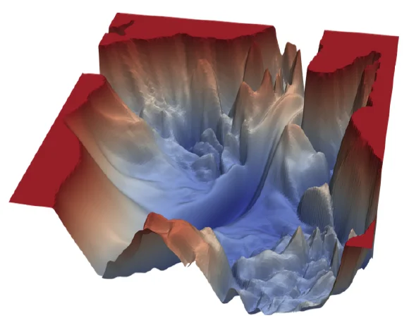
• We want uniform stability of order $o(1/\sqrt{n})$. SGD won’t be stable if it makes super-large steps that cannot be controlled, or if the loss landscape is super-fragmented so we cannot control where we jump. So we need assumptions.

Slide 38: the loss landscape of a neural network (Li et al., NeurIPS 2018, "Visualizing the loss landscape of neural nets").

Beta-smooth functions

Slides 40-41

$\beta$-smooth

A differentiable $f:{\mathbb{R}}^d\to \mathbb{R}$ is $\beta$-smooth if its gradient is $\beta$-Lipschitz:

$$\Vert \nabla f(x)-\nabla f(y)\Vert \le \beta \Vert x-y\Vert$$

Smoothness is good for gradient methods: the gradient changes slowly, so after a small step it does not point in a completely different direction. While $\mu$-strong convexity is a lower bound on the curvature, $\beta$-smoothness is more like an upper bound.

Smooth losses

• Squared loss for linear regression $\ell (w,(x,y))=\frac{1}{2}(⟨x,w⟩-y{)}^2$: convex and smooth with $\beta =\Vert x{\Vert }^2$; if $\Vert x\Vert \le R$ it is $R^2$-smooth. (The slide says “$R$-smoothness”; with $\beta =\Vert x{\Vert }^2$ the constant is $R^2$.)
• Logistic loss $\log (1+\exp (-y{w}^{\top }x))$: the Hessian satisfies ${\nabla }^2\ell \le \text{const}\cdot x{x}^{\top }$, so it is smooth if $\Vert x\Vert$ is bounded.

Stability of gradient descent

Slides 42-47

To minimize $g(w)=\frac{1}{n}{\sum }_i\ell (f_w(x_i),y_i)$: GD uses the full gradient, $w_{t+1}=w_t-\eta \nabla g(w_t)$; SGD samples one point $i$ per step, $w_{t+1}=w_t-\eta \nabla \ell (f_{w_t}(x_i),y_i)$.

Theorem 4 (stability of GD)

Let the loss be continuously differentiable, convex, $\beta$-smooth and $L$-Lipschitz. Run GD with step sizes ${\eta }_t<2/\beta$ for $T$ steps from a fixed $w_0$. Then the solution is uniformly stable with

$${\Delta }_{\sup }\le \frac{2L^2}{n}\sum _{t=1}^T{\eta }_t$$

Proof sketch

Step 1. Compare the trajectories on $S$ and $S^{\prime }$: $w_{t+1}=w_t-{\eta }_t\nabla R_S(w_t)$ and $w_{t+1}^{\prime }=w_t^{\prime }-{\eta }_t\nabla R_{S^{\prime }}(w_t^{\prime })$. Add and subtract ${\eta }_t\nabla R_S(w_t^{\prime })$:

$$\Vert w_{t+1}-w_{t+1}^{\prime }\Vert \le \underset{\text{green: same data set}}{\underbrace{\Vert w_t-w_t^{\prime }-{\eta }_t\nabla R_S(w_t)+{\eta }_t\nabla R_S(w_t^{\prime })\Vert }}+\underset{\text{blue: different data sets}}{\underbrace{{\eta }_t\Vert \nabla R_S(w_t^{\prime })-\nabla R_{S^{\prime }}(w_t^{\prime })\Vert }}$$

Step 2 (blue). $S$ and $S^{\prime }$ differ in one point: only one summand changes, and a gradient at one point changes by at most $2L$, so $\Vert \nabla R_S(w)-\nabla R_{S^{\prime }}(w)\Vert \le 2L/n$.

Step 3 (green). A gradient step with step size $<2/\beta$ on a convex $\beta$-smooth function is non-expansive: $\Vert (w-\eta \nabla R_S(w))-(v-\eta \nabla R_S(v))\Vert \le \Vert w-v\Vert$. This is where the assumptions are used.

Step 4. So $\Vert w_{t+1}-w_{t+1}^{\prime }\Vert \le \Vert w_t-w_t^{\prime }\Vert +{\eta }_t\frac{2L}{n}$. Sum from $t=0$ to $T-1$ with the same start $w_0=w_0^{\prime }$ (the terms telescope): $\Vert w_T-w_T^{\prime }\Vert \le \frac{2L}{n}{\sum }_{t=1}^T{\eta }_t$.

Step 5. Lipschitz: $|\ell (w_T,(x,y))-\ell (w_T^{\prime },(x,y))|\le L\Vert w_T-w_T^{\prime }\Vert \le \frac{2L^2}{n}{\sum }_t{\eta }_t$. $\square$

Stability of SGD

Slides 48-51

Theorem 5 (stability of SGD, convex case)

Same assumptions (continuously differentiable, convex, $\beta$-smooth, $L$-Lipschitz), SGD with step sizes ${\eta }_t<2/\beta$ for $T$ steps:

$${\Delta }_{\sup }(\text{SGD})\le \frac{2L^2}{n}\sum _{t=1}^T{\eta }_t$$

The proof goes along similar lines but is more complicated because of the randomness: GD introduces a small bias at every step; SGD only seldom (when it updates on the changed sample), but then a larger change happens. Details: Hardt, Recht and Singer (and the assignments).

Theorem 6 (stability of SGD, non-convex case)

Assume the loss is $L$-Lipschitz and $\beta$-smooth (not necessarily convex), and run SGD for $T$ steps with decreasing step sizes ${\eta }_t\le c/t$. Then

$${\Delta }_{\sup }\le \frac{1+1/(\beta c)}{n-1}(2c{L}^2{)}^{1/(\beta c+1)}{T}^{\beta c/(\beta c+1)}$$

Ignoring constants:

$${\Delta }_{\sup }\approx \frac{T^{1-1/(\beta c+1)}}{n}$$

Depending on $T$, this can be combined with Theorem 2 to get generalization (but not necessarily consistency).

• These bounds are about stability; they do not yet guarantee consistency (how many steps $T$? convergence to an ERM minimizer?). Hardt, Recht and Singer give some guarantees for the convex setting.

Discussion and more results

Slides 52-53

• The theorems on GD / SGD are the first results about an actual learning algorithm, not just an abstract empirical risk minimizer.
• Depending on the number of steps $T$ we might or might not get stability of order $O(1/\sqrt{n})$, as needed in the generalization bound.
• From the point of view of stability, fewer steps are better (a smaller generalization gap), but this ignores whether we get close enough to the actual minimizer. We revisit this with regularization (Lecture 5).
• Stability has been proved for many algorithms: regularization, many kernel algorithms, GD / SGD in various (also non-convex) scenarios: SGD for deep networks (Hardt, Recht and Singer, ICML 2016), noisy SGD (Pensia, Jog and Loh, 2018), early stopping (Hardt, Ma and Recht, ICLR 2020), sharp vs. flat minima (Wu, Zhu et al., NeurIPS 2020).

Summary

Result	Statement	Assumptions
Proposition 1	$E(R-R_{S_n})(f(S_n))={\Delta }_{av}(A,n)$	none
Theorem 2	$R\le R_{S_n}+{\beta }_n+(2n{\beta }_n+M)\sqrt{\log (1/\delta )/(2n)}$	loss $\le M$; useful iff ${\beta }_n=o(1/\sqrt{n})$
Stability + ERM	consistency	ERM solution uniformly stable
Theorem 3 (ERM)	${\Delta }_{\sup }\le 4L^2/(\mu n)$	$\mu$-strongly convex, $L$-Lipschitz; no complexity of $\mathcal{F}$
Theorems 4, 5 (GD, SGD)	${\Delta }_{\sup }\le \frac{2L^2}{n}{\sum }_{t\le T}{\eta }_t$	convex, $\beta$-smooth, $L$-Lipschitz, ${\eta }_t<2/\beta$
Theorem 6 (SGD)	${\Delta }_{\sup }\approx T^{1-1/(\beta c+1)}/n$	non-convex, ${\eta }_t\le c/t$

Self-Test

Question cards (12)

What is the stability principle, and why is it an alternative to capacity bounds?

Answer

If the output of an algorithm changes only a little when one training point is replaced, the algorithm generalizes. It analyses the actual algorithm instead of giving worst-case guarantees over all functions of a class.

Define $S_n^i$, average stability and uniform stability.

Answer

$S_n^i$ is $S_n$ with $Z_i$ replaced by an independent $Z_i^{\prime }$. ${\Delta }_{av}=E\frac{1}{n}{\sum }_i(\ell (f(S_n),Z_i^{\prime })-\ell (f(S_n^i),Z_i^{\prime }))$. ${\Delta }_{\sup }={\sup }_{i,S_n,S_n^i,Z}|\ell (f(S_n),Z)-\ell (f(S_n^i),Z)|$. Always ${\Delta }_{av}\le {\Delta }_{\sup }$.

State and prove Proposition 1.

Answer

$E(R(f(S_n))-R_{S_n}(f(S_n)))={\Delta }_{av}$. Write $ER(f(S_n))=E\frac{1}{n}{\sum }_i\ell (f(S_n),z_i^{\prime })$ with test points $z_i^{\prime }$, and $E{R}_{S_n}(f(S_n))=E\frac{1}{n}{\sum }_i\ell (f(S_n),z_i)=E\frac{1}{n}{\sum }_i\ell (f(S_n^i),z_i^{\prime })$ by exchanging $z_i$ and $z_i^{\prime }$; subtract.

State Theorem 2 and the tool used in its proof.

Answer

For loss bounded by $M$ and ${\beta }_n={\Delta }_{\sup }$: w.p. $1-\delta$, $R(f(S_n))\le R_{S_n}(f(S_n))+{\beta }_n+(2n{\beta }_n+M)\sqrt{\log (1/\delta )/(2n)}$. McDiarmid applied to $\phi (S)=R(f(S))-R_S(f(S))$ with bounded differences $2{\beta }_n+M/n$, plus $E\phi ={\Delta }_{av}\le {\beta }_n$.

Which uniform stability rates make Theorem 2 useful, and why?

Answer

${\beta }_n=o(1/\sqrt{n})$: the term $2n{\beta }_n\sqrt{\log (1/\delta )/(2n)}$ behaves like $\sqrt{n}{\beta }_n$. $1/n$ works, $1/\sqrt{n}$ gives a constant gap.

Why does stability alone not give consistency, and what does?

Answer

A constant predictor is perfectly stable but not the best in $\mathcal{F}$. With ERM: $R(f_n)-R(f_{\mathcal{F}})=[R(f_n)-R_n(f_n)]+[R_n(f_n)-R_n(f_{\mathcal{F}})]+[R_n(f_{\mathcal{F}})-R(f_{\mathcal{F}})]$: small by stability, $\le 0$ by minimization, small by the LLN.

Define $\mu$-strong convexity and give the 1d intuition.

Answer

$f(y)\ge f(x)+\nabla f(x)(y-x)+\frac{\mu }{2}\Vert y-x{\Vert }^2$. In 1d: $f^{\prime \prime }\ge \mu$, a lower bound on the curvature; in ${\mathbb{R}}^d$ the smallest Hessian eigenvalue is $\ge \mu$.

State Theorem 3 and sketch its proof.

Answer

$\mu$-strongly convex and $L$-Lipschitz loss: ${\Delta }_{\sup }(ERM)\le 4L^2/(\mu n)$. Strong convexity gives $\frac{\mu }{2}\Vert w_S-w_{S^{\prime }}{\Vert }^2\le R_S(w_{S^{\prime }})-R_S(w_S)\le \frac{2L}{n}\Vert w_S-w_{S^{\prime }}\Vert$, so $\Vert w_S-w_{S^{\prime }}\Vert \le 4L/(\mu n)$; Lipschitz gives another factor $L$.

Why is the squared loss of a linear model not strongly convex, and how is this fixed?

Answer

Its Hessian $2x{x}^{\top }$ has rank 1, so for $d>1$ the smallest eigenvalue is 0. Adding $\lambda \Vert w{\Vert }^2$ makes it $2\lambda$-strongly convex (ridge regression).

Define $\beta$-smoothness and compare it with strong convexity.

Answer

$\Vert \nabla f(x)-\nabla f(y)\Vert \le \beta \Vert x-y\Vert$: the gradient is $\beta$-Lipschitz, an upper bound on the curvature; strong convexity is a lower bound.

State the stability bound for GD and the key steps of its proof.

Answer

Convex, $\beta$-smooth, $L$-Lipschitz, ${\eta }_t<2/\beta$: ${\Delta }_{\sup }\le \frac{2L^2}{n}{\sum }_t{\eta }_t$. The gradients on $S$ and $S^{\prime }$ differ by at most $2L/n$; a gradient step is non-expansive; so the distance grows by at most ${\eta }_{t}2L/n$ per step; sum and apply Lipschitz.

What does the SGD stability bound say about the number of training steps?

Answer

The bound grows with ${\sum }_t{\eta }_t$ (convex) or $T^{1-1/(\beta c+1)}$ (non-convex): fewer steps give more stability and a smaller generalization gap, but maybe not a good minimizer. With constant step size, Theorem 2 needs $T=o(\sqrt{n})$.

Multiple Choice

Multiple choice (7)

Which relation between the two stability notions always holds?

• ${\Delta }_{\sup }(A,n)\le {\Delta }_{av}(A,n)$

• ${\Delta }_{av}(A,n)\le {\Delta }_{\sup }(A,n)$

• ${\Delta }_{av}(A,n)={\Delta }_{\sup }(A,n)/n$

• they are unrelated

Explanation

An average of loss differences is at most their supremum (slide 10).

Proposition 1 states that the expected generalization gap $E(R(f(S_n))-R_{S_n}(f(S_n)))$

• is at most $2/n$ for every algorithm

• equals the average stability ${\Delta }_{av}(A,n)$

• equals the uniform stability ${\Delta }_{\sup }(A,n)$

• is 0 for ERM

Explanation

Exactly ${\Delta }_{av}$, which is at most ${\Delta }_{\sup }$. ERM usually has a positive gap (the training error is optimistic).

An algorithm has uniform stability ${\beta }_n=1/\sqrt{n}$ and loss bound $M$. What does Theorem 2 give?

• a gap of order $1/n$

• a gap of order $1/\sqrt{n}$

• a gap that does not go to 0

• consistency

Explanation

$2n{\beta }_n\sqrt{\log (1/\delta )/(2n)}=\sqrt{2\log (1/\delta )}$ is a constant; one needs ${\beta }_n=o(1/\sqrt{n})$.

Which statement about stability and consistency is true?

• Every uniformly stable algorithm is consistent.

• A constant predictor is perfectly stable but in general not consistent.

• Consistent algorithms are always uniformly stable at rate $1/n$.

• Stability implies that the approximation error is 0.

Explanation

Slide 21. Stability controls the gap between training and test error; consistency needs in addition that the empirical risk is (approximately) minimized.

Which assumptions does Theorem 3 ( ${\Delta }_{\sup }(ERM)\le 4L^2/(\mu n)$) need?

• finite VC dimension of $\mathcal{F}$

• a loss that is $\mu$-strongly convex and $L$-Lipschitz in the parameters

• a $\beta$-smooth loss and step sizes $<2/\beta$

• linearly separable data

Explanation

The complexity of $\mathcal{F}$ does not appear at all. Smoothness and step sizes are the assumptions of the GD/SGD theorems.

For GD on a convex, $\beta$-smooth, $L$-Lipschitz loss, the stability bound $\frac{2L^2}{n}{\sum }_{t=1}^T{\eta }_t$ suggests that

• running fewer steps (or with smaller steps) makes the solution more stable

• running more steps always improves generalization

• the step size does not matter

• the bound is independent of $n$

Explanation

The bound grows with the total step length; this supports early stopping, at the price of possibly not reaching a good minimizer.

Why is 1-nearest neighbour not uniformly stable at rate $1/n$?

• because it has infinite VC dimension

• because replacing a single training point can flip the prediction at a test point, changing the loss by 1

• because its loss is not bounded

• because it is not an ERM algorithm

Explanation

Sheet 5: uniform stability is a supremum over all samples and test points, and one point can be the nearest neighbour of the test point. On average the effect is only $1/n$.

References

All sources cited on the slides, in slide order (13 entries)

Slide	Source	Key point
3	Hardt and Recht, Patterns, Predictions, and Actions, Sec. 6.4 (online)	stability
3	Mohri, Rostamizadeh and Talwalkar, Foundations of Machine Learning, Sec. 11.2	stability bounds (full proof of Theorem 2, p. 268)
3	Shalev-Shwartz and Ben-David, Understanding Machine Learning, Sec. 13.2 (online)	stability and regularization
3	Bousquet and Elisseeff, “Stability and generalization”, JMLR, 2002	the standard uniform stability bound
3	Shalev-Shwartz, Shamir, Srebro and Sridharan, “Learnability, Stability and Uniform Convergence”, JMLR, 2010	stability is sufficient and necessary for learning
3, 36, 53	Hardt, Recht and Singer, “Train faster, generalize better: Stability of stochastic gradient descent”, ICML 2016	stability of SGD
11	Mohri textbook	stability implies generalization
23	Hardt and Recht, Chapter 6, p. 111, Theorem 4	ERM with strongly convex loss is stable
36	Hardt and Recht, Chapter 6, Theorem 6, p. 120	stability of (S)GD
38	Li et al., “Visualizing the loss landscape of neural nets”, NeurIPS 2018	loss landscape figure
53	Pensia, Jog and Loh, “Stability of stochastic gradient descent on non-convex losses”, arXiv 2018	noisy SGD
53	Hardt, Ma and Recht, “Identity matters in deep learning”, ICLR 2020	stability and early stopping
53	Wu, Zhu et al., “Understanding SGD generalization in deep learning via stability”, NeurIPS 2020	sharp vs. flat minima

Related

• Previous: Lecture 3: Statistical Learning Theory · Course: Overview
• Concepts: Algorithmic Stability, Strong Convexity, Smoothness, Stochastic Gradient Descent, Hoeffding Inequality (McDiarmid), Leave-One-Out Error
• Exercises: Sheet 5 (stability of 1-NN, the averaging algorithm, one-pass SGD)