Lecture 3: Statistical Learning Theory

TL;DR

1. Setup: ERM over a function class $\mathcal{F}$ chosen in advance. Consistency w.r.t. $\mathcal{F}$ means $R(f_n)\to R(f_{\mathcal{F}})$: it concerns only the estimation error. The question is when ERM succeeds, and the answer is: when the complexity of $\mathcal{F}$ is under control.
2. Hoeffding: for independent $Z_i\in [0,1]$, $P(|S_n-E(S_n)|\ge \epsilon )\le 2\exp (-2n{\epsilon }^2)$. For a fixed function this gives $|R(f_0)-R_n(f_0)|\le \sqrt{\log (1/\delta )/(2n)}$: error $\sim 1/\sqrt{n}$, sample size $\sim 1/{\epsilon }^2$.
3. Uniform convergence $P({\sup }_{f\in \mathcal{F}}|R(f)-R_n(f)|>\epsilon )\to 0$ is sufficient and necessary for the consistency of ERM (Vapnik and Chervonenkis 1971).
4. Finite class with $m$ functions (union bound): $R(f)\le R_n(f)+\sqrt{(\log (2m)+\log (1/\delta ))/(2n)}$ for all $f\in \mathcal{F}$. We pay only $\log m$.
5. Infinite classes: replace $m$ by the shattering coefficient $\mathcal{N}(\mathcal{F},2n)$ (symmetrization with a ghost sample). The VC dimension is the largest $n$ with $\mathcal{N}(\mathcal{F},n)=2^n$. Sauer-Shelah: $\mathcal{N}(\mathcal{F},n)\le {\sum }_{i=0}^d\left(\genfrac{}{}{0ex}{}{n}{i}\right)\le (en/d{)}^d$, so the growth function is either $2^n$ or polynomial. Bound: $R(f)\le R_n(f)+2\sqrt{(d\log (2en/d)-\log \delta )/n}$; ERM is consistent iff $\mathrm{VC}(\mathcal{F})<\infty$.
6. VC of linear classifiers in ${\mathbb{R}}^d$: $d+1$. With margin $\rho$ on data in a ball of radius $R$: $\min \{R^2/{\rho }^2,d+1\}$, dimension-free. Neural networks: $O(W\log W)$. Rademacher complexity measures how well $\mathcal{F}$ fits random labels. In the overparameterized regime all these bounds are vacuous.

Exam relevance

• Real exam, task type “VC dimension and growth function” (4 P): a table of values $N(\mathcal{F},n)$; read off the VC dimension and decide which rows are valid or impossible growth functions (Sauer-Shelah, monotonicity, $\le 2^n$). Train it with the task and part 3 of the widget.
• Real exam, task type “bounds” (4 P): select which function or rate satisfies a condition (does it go to 0, at which rate). See this task.
• Mock exam: MC on comparing two bounds (rates $\sqrt{d\ln n/n}$ vs. $d\ln n/n$) and on Sauer-Shelah; a longer task on the VC dimension of intervals and unions of two intervals (Sheet 4, Exercise 2).
• Sheet 3: Hoeffding sample sizes (Exercise 1) and validating $m$ classifiers at once with a union bound (Exercise 2). Sheet 4, Exercise 3: VC bounds for one-vs-all multiclass classification.

Overview: 1. Setup and consistency w.r.t. $\mathcal{F}$, 2. Concentration inequalities, 3. The error of a fixed function and uniform convergence, 4. Finite classes, 5. Infinite classes: shattering coefficient, growth function, 6. VC dimension, 7. Rademacher complexity, 8. Limitations and outlook.

Statistical learning theory

Setup

Slides 3-5

(Literature: von Luxburg and Schölkopf 2011 for a high-level overview; Bousquet, Boucheron and Lugosi 2003 more technical; Devroye, Györfi and Lugosi 1996 the classical book; Shalev-Shwartz and Ben-David less technical, Bach pretty technical.)

We consider the standard setup: an unknown distribution $P$ generates the data, and we look at binary classification, typically with the 0-1 loss (the maths is simpler; many results hold more generally). The training data is i.i.d. from $P$. Because we do not know $P$, we perform ERM over a fixed function class $\mathcal{F}$ chosen in advance, before seeing the data. We do not ask how to solve the optimization problem; we assume we always find an empirical risk minimizer. We ask under which conditions this approach is “successful”. One approach that leads to successful learning consists in bounding the complexity of the function class $\mathcal{F}$.

Consistency with respect to the function class

Slides 6-7

Notation: $f^{\ast }$ is the Bayes classifier, $f_{\mathcal{F}}={\mathrm{argmin}}_{f\in \mathcal{F}}R(f)$ the best classifier in $\mathcal{F}$, and $f_n$ the classifier chosen from $\mathcal{F}$ on a sample of $n$ points.

Three kinds of consistency

1. Consistent with respect to $\mathcal{F}$ and $P$: $\forall \epsilon >0:P(R(f_n)-R(f_{\mathcal{F}})>\epsilon )\to 0$ as $n\to \infty$.
2. Bayes-consistent with respect to $P$: $\forall \epsilon >0:P(R(f_n)-R(f^{\ast })>\epsilon )\to 0$ as $n\to \infty$.
3. Universally consistent with respect to $\mathcal{F}$ (resp. universally Bayes-consistent): consistent w.r.t. $\mathcal{F}$ (resp. Bayes-consistent) for all $P$.

Trap

Consistency with respect to a fixed $\mathcal{F}$ only concerns the estimation error $R(f_n)-R(f_{\mathcal{F}})$, not the approximation error. All bounds in this lecture control the estimation error. (In Lecture 1.2, $f_{\mathcal{F}}$ was written $\tilde{f}$.)

Concentration inequalities

From the law of large numbers to concentration

Slides 8-10

(Literature: Bach Sec. 1.2; Hoeffding in every learning theory book; McDiarmid 1989; the book Concentration Inequalities by Boucheron, Lugosi and Massart.)

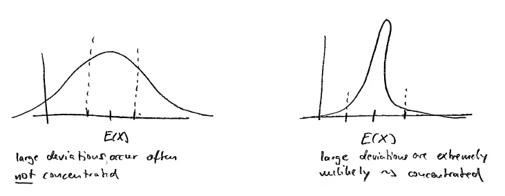
The LLN (Proposition 1: $S_n:=\frac{1}{n}{\sum }_{i=1}^n{Z}_i\to E(Z)$ almost surely) is qualitative. In learning theory we want quantitative versions: how far is the empirical average from the true one, and with which probability? Such statements are concentration inequalities:

$$P(|S_n-E(S_n)|\ge \epsilon )\le \delta (\epsilon )$$

where $\delta (\epsilon )$ goes to 0 very fast as $\epsilon$ grows.

Slide 10: not concentrated (left) and concentrated (right) around E(X).

Hoeffding’s inequality

Slides 11-12

Proposition 2 (Chernoff 1952, Hoeffding 1963)

Let $Z_1,\dots ,Z_n$ be independent random variables with values in $[0,1]$. Then for any $\epsilon >0$,

$$P(|S_n-E(S_n)|\ge \epsilon )\le 2\exp (-2n{\epsilon }^2)$$

(Proof skipped.)

• The random variables do not need to have the same distribution, as long as their range (more generally, their variance) is controlled.
• Independence is crucial.
• Whenever you want to prove concentration, Hoeffding is always the first thing to try.
• It is tight in some situations (fair coin tosses) and not so tight in others; if you know more about the variables, other inequalities may be better.

Mini example: coin tosses

$n=100$ fair coin tosses, $\epsilon =0.1$: the frequency of heads deviates from $0.5$ by at least $0.1$ with probability at most $2e^{-2\cdot 100\cdot 0.01}=2e^{-2}\approx 0.27$. With $n=1000$: $2e^{-20}\approx 4\cdot 10^{-9}$. Ten times more data makes the exponent ten times larger.

McDiarmid’s inequality

Slides 13-14

Theorem 3 (McDiarmid, bounded differences inequality)

Let $f:{\mathcal{X}}^n\to \mathbb{R}$ and assume there are constants $c_1,\dots ,c_n>0$ such that for all $x_1,\dots ,x_n\in \mathcal{X}$ and $x_i^{\prime }\in \mathcal{X}$:

$$|f(x_1,\dots ,x_i,\dots ,x_n)-f(x_1,\dots ,x_i^{\prime },\dots ,x_n)|\le c_i$$

Let $X_1,\dots ,X_n$ be independent. Then

$$P\left(\right|f(X_1,\dots ,X_n)-E(f(X_1,\dots ,X_n))|\ge \epsilon )\le 2\exp \left(\frac{-2{\epsilon }^2}{{\sum }_{i=1}^n{c}_i^2}\right)$$

Hoeffding as a special case

Take $f(z_1,\dots ,z_n)=\frac{1}{n}{\sum }_i{z}_i$ with $z_i\in [0,1]$. Changing one coordinate changes $f$ by at most $c_i=1/n$, so ${\sum }_i{c}_i^2=n\cdot 1/n^2=1/n$ and the bound becomes $2\exp (-2n{\epsilon }^2)$: Hoeffding. McDiarmid is super useful beyond learning theory (randomized algorithms) and comes back in the section on stability (Lecture 4).

Controlling the estimation error: generalization bounds

The error of a fixed function

Slides 15-20

For a fixed function we saw strong consistency from the LLN (Lecture 1.2). Hoeffding gives a sharper result:

Proposition 4 (error in measuring the risk of a fixed function)

Fix $f_0\in \mathcal{F}$ and consider a bounded loss. Then

$$P(|R_n(f_0)-R(f_0)|\ge \epsilon )\le \exp (-2n{\epsilon }^2)$$

Proof

Apply Hoeffding to $Z_i=\ell (X_i,Y_i,f_0(X_i))$: independent, bounded, with mean $R(f_0)$. This gives convergence in probability (weak consistency). For almost sure convergence, apply the Borel-Cantelli lemma: the key is that ${\sum }_{n=1}^{\infty }\exp (-2n{\epsilon }^2)<\infty$. $\square$

The same statement as a generalization bound

Fix an error probability $\delta$ (say 0.05), set $\delta =\exp (-2n{\epsilon }^2)$ and solve for $\epsilon$: with probability at least $1-\delta$,

$$|R(f_0)-R_n(f_0)|\le \sqrt{\frac{\log (1/\delta )}{2n}}$$

The factor 2

Hoeffding for the two-sided event $|\cdot |\ge \epsilon$ has the factor 2: $2\exp (-2n{\epsilon }^2)$, which gives $\sqrt{\log (2/\delta )/(2n)}$. Proposition 4 on slide 17 drops it; the finite-class bound (slide 29) keeps it. In a computation, use $2\exp (-2n{\epsilon }^2)$ unless the task says otherwise.

Sample complexity of error estimation

• Error at most $\epsilon$ with a fixed small failure probability needs $n{\epsilon }^2=O(1)$, i.e. $n=O(1/{\epsilon }^2)$.
• The error with $n$ sample points scales as $1/\sqrt{n}$.

If you already fixed $f_0$ (by some complicated training) and want to estimate its test error up to $\epsilon =1\%$ on a fresh test set, you need of the order $1/{\epsilon }^2=10,000$ test points. It is impossible to beat or trick these numbers.

Uniform convergence

Slides 21-25

The bound holds only for a fixed $f_0$, and we saw that this does not make ERM consistent. Idea: require that the empirical risk is close to the true risk for all functions in $\mathcal{F}$ simultaneously. Then it is also close for the function $f_n$ the algorithm picks.

Definition 5 (uniform convergence)

$R_n(f)$ converges to $R(f)$ uniformly over $\mathcal{F}$ (the law of large numbers holds uniformly over $\mathcal{F}$) if

$$\forall \epsilon >0:\underset{n\to \infty }{\lim }P(\underset{f\in \mathcal{F}}{\sup }|R_n(f)-R(f)|>\epsilon )=0$$

Proposition 6 (uniform convergence is sufficient for consistency)

Let $f_n$ minimize the empirical risk in $\mathcal{F}$. Then

$$P(|R(f_n)-R(f_{\mathcal{F}})|\ge \epsilon )\le P(\underset{f\in \mathcal{F}}{\sup }|R(f)-R_n(f)|\ge \epsilon /2)$$

Proof

By definition of $f_{\mathcal{F}}$, $R(f_n)-R(f_{\mathcal{F}})\ge 0$. Insert and subtract empirical risks:

$$\begin{array}{rl}|R(f_n)-R(f_{\mathcal{F}})|& =R(f_n)-R_n(f_n)+\underset{\le 0\text{ by def. of }{f}_n}{\underbrace{R_n(f_n)-R_n(f_{\mathcal{F}})}}+R_n(f_{\mathcal{F}})-R(f_{\mathcal{F}})\\ & \le (R(f_n)-R_n(f_n))+(R_n(f_{\mathcal{F}})-R(f_{\mathcal{F}}))\le 2\underset{f\in \mathcal{F}}{\sup }|R(f)-R_n(f)|\end{array}$$

So $|R(f_n)-R(f_{\mathcal{F}})|\ge \epsilon$ implies ${\sup }_f|R(f)-R_n(f)|\ge \epsilon /2$. $\square$

Uniform convergence is necessary

Slides 26-27

Theorem 7 (Vapnik and Chervonenkis 1971)

Let $\mathcal{F}$ be any function class. Then ERM is uniformly consistent with respect to $\mathcal{F}$ if and only if uniform convergence holds:

$$P(\underset{f\in \mathcal{F}}{\sup }|R(f)-R_n(f)|>\epsilon )\to 0\text{as }n\to \infty$$

The proof is beyond the scope of the lecture; the “necessary” direction is a very deep result.

The big question now: how do we know whether uniform convergence holds for a function class $\mathcal{F}$?

Generalization bound for finite classes

Capacity measures

Slides 28-29

• If $\mathcal{F}$ is too large (the counterexample in Lecture 1.2), there is no uniform convergence.
• If $\mathcal{F}$ is small (a single function), there is uniform convergence.

We want to measure the size of a function class in a way that bounds $P({\sup }_{f\in \mathcal{F}}|R(f)-R_n(f)|>\epsilon )$.

The union bound for finitely many functions

Slides 30-33

For $\mathcal{F}=\{f_1,\dots ,f_m\}$ and Hoeffding for each $f_i$:

$$\begin{array}{rl}P(\underset{f\in \mathcal{F}}{\sup }|R(f)-R_n(f)|\ge \epsilon )& =P(|R(f_1)-R_n(f_1)|\ge \epsilon \text{ or }\dots \\ & \text{ or }|R(f_m)-R_n(f_m)|\ge \epsilon )\\ & \le \sum _{i=1}^{m}P(|R(f_i)-R_n(f_i)|\ge \epsilon )\le 2m\exp (-2n{\epsilon }^2)\end{array}$$

Proposition 8 and Theorem 9 (generalization bound for finite classes)

Let $\mathcal{F}$ be finite with $m$ functions. For $0<\epsilon <1$: with probability at least $1-2m\exp (-2n{\epsilon }^2)$, $|R(f)-R_n(f)|<\epsilon$ for all $f\in \mathcal{F}$. Setting $\delta =2m\exp (-2n{\epsilon }^2)$: with probability at least $1-\delta$, for all $f\in \mathcal{F}$

$$R(f)\le R_n(f)+\sqrt{\frac{\log (2m)+\log (1/\delta )}{2n}}$$

Digesting the bound

• True risk $\le$ empirical risk + a “capacity term”.
• A larger class (larger $m$) gives a worse bound, but only logarithmically in $m$. The rate is again $1/\sqrt{n}$: the error scales as $\sqrt{(\log m)/n}$.
• The bound holds uniformly for all $f\in \mathcal{F}$, so in particular for the function the algorithm picks based on the data.
• If you let the class grow with $n$ to fit better, you need $(\log m)/n\to 0$ for consistency.

The bound for a fixed function, for a finite class of m functions and for a class of VC dimension d, against n on log-log axes. The dots mark the sample size needed for the target accuracy ε. Move m, d and δ.

Task: Hoeffding and sample sizes

Exam-style task: how many validation points? (4 P)

Use $P(|R_n(f)-R(f)|\ge \epsilon )\le 2\exp (-2n{\epsilon }^2)$ for a fixed $f$.

(a) (1 P, easy) How many test points guarantee $|R_n(f)-R(f)|<0.02$ with probability at least $0.95$ for one fixed classifier?

(b) (1.5 P, harder) You validate $m=100$ classifiers on the same test set and want the guarantee for all of them simultaneously. How many points now?

(c) (1.5 P, transfer) By which factor does the answer of (a) change if $\epsilon$ is halved? And the answer of (b) if $m$ is squared to $10,000$?

Solution

(a) $2e^{-2n{\epsilon }^2}\le \delta ⟺n\ge \frac{\log (2/\delta )}{2{\epsilon }^2}=\frac{\ln 40}{2\cdot 0.0004}=\frac{3.689}{0.0008}\approx 4611.2$, so $n=4612$. (1 P)

(b) Union bound: $2m{e}^{-2n{\epsilon }^2}\le \delta ⟺n\ge \frac{\log (2m)+\log (1/\delta )}{2{\epsilon }^2}=\frac{\ln 200+\ln 20}{0.0008}=\frac{5.298+2.996}{0.0008}\approx 10367.5$, so $n=10368$. About $2.2$ times (a), not 100 times. (1.5 P)

(c) $n\propto 1/{\epsilon }^2$: halving $\epsilon$ quadruples $n$. Squaring $m$ doubles $\log m$: $n\ge (\ln 20000+\ln 20)/0.0008=(9.903+2.996)/0.0008\approx 16124$, only about $1.6$ times more. (1.5 P)

Example: partitioning-based estimators

Slides 34-42

Split $\mathcal{X}=[0,1]$ into a grid of $k$ cells of equal size and let ${\mathcal{F}}_k$ be all functions that are piecewise constant (0 or 1) on the cells. $|{\mathcal{F}}_k|=2^k$.

Slide 35: a piecewise constant function on k grid cells.

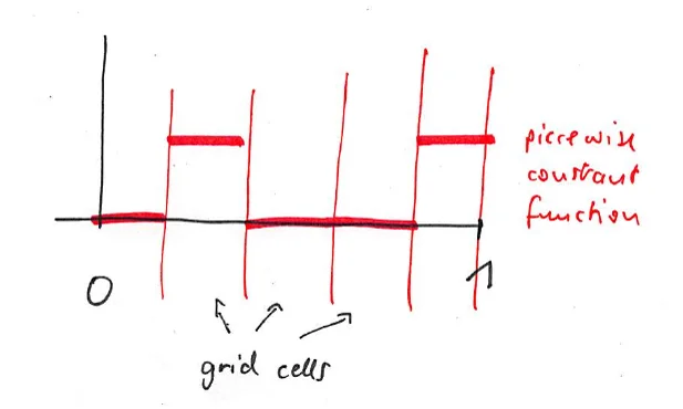
How should $k$ depend on $n$?

• $k=1$: the estimation error converges to 0 very quickly (two functions), but the approximation error stays large (a constant cannot approximate the Bayes classifier).
• $k\approx n$ or larger: the estimation error is large (about one point per cell), the approximation error might be small.
• Intuition: to get the estimation error to 0 we need “infinitely many points” in each cell; to get the approximation error to 0 we need ever finer cells.

Consistency of partitioning estimators

• $k$ fixed: the key term is $\log (m)/n=\log (2^k)/n\approx k/n\to 0$: ERM is uniformly consistent w.r.t. ${\mathcal{F}}_k$ (estimation error $\to 0$), but not Bayes-consistent in general.
• $k=k(n)$ growing: consistency w.r.t. ${\mathcal{F}}_{k(n)}$ needs $k(n)/n\to 0$ (for example $k(n)=\log n$): there are about $n/k\to \infty$ points per cell. For Bayes consistency we additionally need $k\to \infty$ (plus regularity of $P$, so that it can be approximated by histograms).
• In $d$ dimensions: $k^d$ cells, $2^{k^d}$ functions, error term $\approx k^d/n$: exponentially many samples in $d$. Not a very practical idea.

Trap

These results only hold if the partition is formed independently of the data. For data-dependent partitions (kNN, decision trees, random forests) one needs different techniques.

Infinite classes: shattering coefficient and growth function

Why the finite bound fails

Slides 43-44

For finite classes we measure the size by the number $m$ of functions, which gives a bound with plausible behaviour. For an infinite class (all linear functions, say) $m=\infty$ and the union bound gives nothing.

The shattering coefficient

Slides 45-48

Shattering coefficient

For a sample $X_1,\dots ,X_n$ let ${\mathcal{F}}_{X_1,\dots ,X_n}:=\{f{|}_{X_1,\dots ,X_n}:f\in \mathcal{F}\}$ be the restrictions of the functions to the sample (the labelings $\mathcal{F}$ can produce on it). The shattering coefficient is the maximal number of such labelings:

$$\mathcal{N}(\mathcal{F},n):=\max \{|{\mathcal{F}}_{X_1,\dots ,X_n}|:X_1,\dots ,X_n\in \mathcal{X}\}$$

Slide 46: 𝓕 = half-lines [a, ∞) on ℝ realizes only 4 of 8 labelings of three points: 𝒩(𝓕, 3) = 4. In general 𝒩(𝓕, n) = n + 1.

Slide 47: positive class = above a horizontal line. The count depends on the data set; the maximum over data sets is 𝒩(𝓕, 5) = 6.

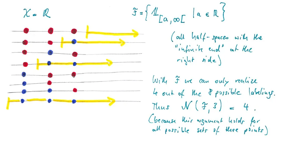
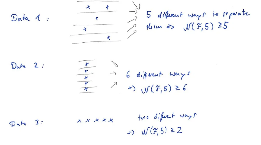
Example 3 (slide 48): $\mathcal{X}={\mathbb{R}}^2$, $\mathcal{F}$ = interiors of circles. Question: can you bound the shattering coefficient for small $n$?

Generalization bound with the shattering coefficient

Slides 49-53

Theorem 10 (generalization bound with the shattering coefficient)

Let $\mathcal{F}$ be any function class. For all $0<\epsilon <1$:

$$P(\underset{f\in \mathcal{F}}{\sup }|R(f)-R_n(f)|>\epsilon )\le 2\mathcal{N}(\mathcal{F},2n)\exp (-n{\epsilon }^2/4)$$

The other way round: with probability at least $1-\delta$, all $f\in \mathcal{F}$ satisfy

$$R(f)\le R_n(f)+2\sqrt{\frac{\log (\mathcal{N}(\mathcal{F},2n))-\log (\delta )}{n}}$$

Proof by symmetrization

Let $R_n$ be the risk on the given sample and $R_n^{\prime }$ the risk on a second, independent sample of $n$ points, the ghost sample.

Proposition 11 (symmetrization lemma): $P({\sup }_f|R(f)-R_n(f)|>\epsilon )\le 2P({\sup }_f|R_n(f)-R_n^{\prime }(f)|>\epsilon /2)$ (elementary proof, omitted).

The point of symmetrization: the right-hand side depends only on the values of the functions on the $2n$ sample points. If $f$ and $g$ agree on the original and the ghost sample, then $R_n(f)=R_n(g)$ and $R_n^{\prime }(f)=R_n^{\prime }(g)$. So the supremum runs over finitely many functions: all binary labelings of the two samples, at most $\mathcal{N}(\mathcal{F},2n)$ of them ($2n$ because of $n$ original and $n$ ghost points). Now Theorem 10 is a consequence of the finite-class argument (Theorem 9). $\square$

Discussion

• The bound is the finite-class bound with $m$ replaced by the shattering coefficient.
• The shattering coefficient measures how powerful a class is: how many different labelings of a data set it can realize. Overfitting happens if the class can fit everything; then the shattering coefficient is large and there is no consistency.
• For consistency we need $\log \mathcal{N}(\mathcal{F},2n)/n\to 0$: the number of labelings has to grow at most polynomially in $n$ (sub-exponentially).
• Shattering coefficients are complicated to compute. The VC dimension below is the tool that tells us how fast they grow.

The growth function

Slide 54

Growth function

To stress how the shattering coefficient behaves with $n$, one also calls it the growth function: $S_{\mathcal{F}}(n):\mathbb{N}\to \mathbb{N},n\mapsto \mathcal{N}(\mathcal{F},n)$. Another common notation is ${\Pi }_{\mathcal{F}}(n)$.

Properties every growth function has (for exam tables)

• $\mathcal{N}(\mathcal{F},0)=1$ (the empty set has one labeling) and $1\le \mathcal{N}(\mathcal{F},n)\le 2^n$.
• Non-decreasing: $\mathcal{N}(\mathcal{F},n+1)\ge \mathcal{N}(\mathcal{F},n)$, since every labeling of $n+1$ points restricts to a labeling of $n$ of them.
• At most doubling: $\mathcal{N}(\mathcal{F},n+1)\le 2\mathcal{N}(\mathcal{F},n)$, since each labeling of $n$ points extends in at most two ways.
• Once $\mathcal{N}(\mathcal{F},k)<2^k$, also $\mathcal{N}(\mathcal{F},n)<2^n$ for all $n\ge k$ (a subset of a shattered set is shattered), and Sauer-Shelah bounds all values by ${\sum }_{i=0}^d\left(\genfrac{}{}{0ex}{}{n}{i}\right)$ with $d$ the VC dimension.

1: all labelings of n points on the line, and which ones a class realizes. 2: the growth function against 2ⁿ and the Sauer-Shelah bound. 3: type a row of an exam table and check whether it can be a growth function.

VC dimension

Definition and examples

Slides 55-62

Shattering and VC dimension

$\mathcal{F}$ shatters a set of points $X_1,\dots ,X_n$ if it can realize all labelings: $|{\mathcal{F}}_{X_1,\dots ,X_n}|=2^n$. The VC dimension is the largest $n$ such that there exists a sample of size $n$ that is shattered:

$$\mathrm{VC}(\mathcal{F})=\max \{n\in \mathbb{N}\mid \exists X_1,\dots ,X_n\in \mathcal{X}\text{ s.t. }|{\mathcal{F}}_{X_1,\dots ,X_n}|=2^n\}$$

If the maximum does not exist, $\mathrm{VC}(\mathcal{F})=\infty$. (VC stands for Vapnik and Chervonenkis.)

"There exists" vs. "for all"

• To show $\mathrm{VC}\ge n$: find one set of $n$ points that is shattered.
• To show $\mathrm{VC}<n+1$: show that no set of $n+1$ points is shattered (for every configuration, give a labeling that cannot be realized).

Some sets of size $\le \mathrm{VC}$ may not be shattered (four points on a line cannot be shattered by rectangles), and that does not matter.

Slide 58: closed intervals [a, b] on ℝ. Two points are shattered; for three points, (+, −, +) is impossible. VC = 2.

Slide 59: axis-parallel rectangles in ℝ². A diamond of 4 points is shattered (VC ≥ 4). Among 5 points one is not extreme in both axis directions; label it − and the others +: impossible. VC = 4.

Slide 60: convex polygons with d corners in ℝ² have VC = 2d + 1. Lower bound: 2d + 1 points on a circle can be shattered (few red points: take their polygon; many red points: cut off the blue ones).

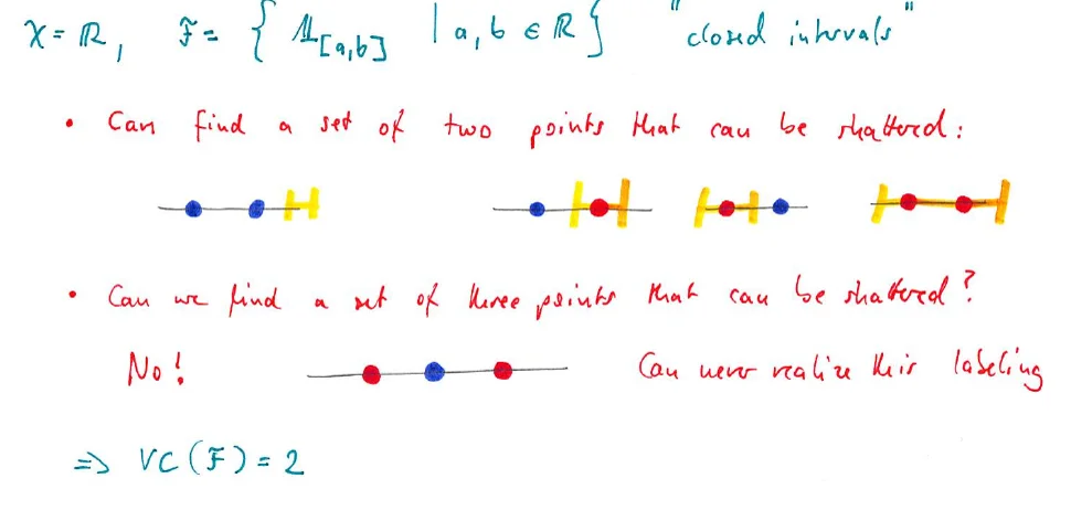
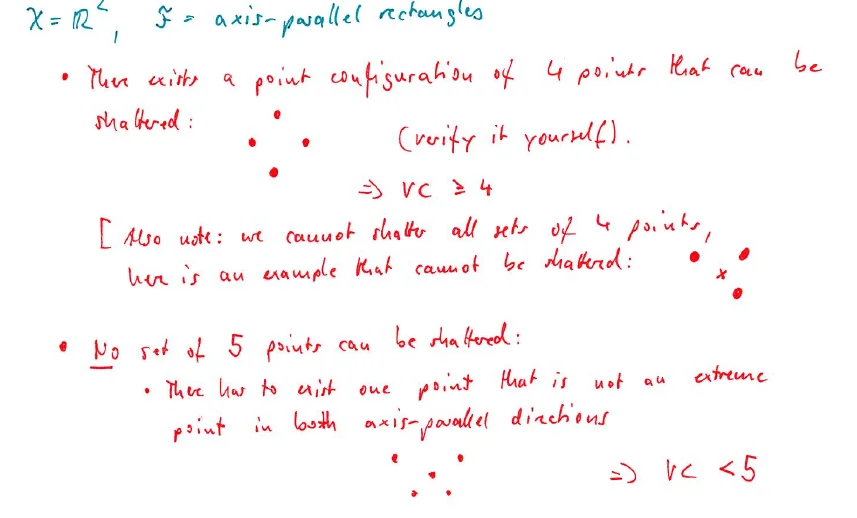
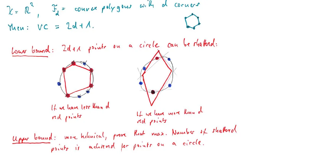
VC dimensions to know

Class	VC dimension
half-lines $1_{[a,\infty )}$ on $\mathbb{R}$	1
closed intervals $1_{[a,b]}$ on $\mathbb{R}$	2
unions of at most two intervals (Sheet 4, mock)	4
axis-parallel rectangles in ${\mathbb{R}}^2$	4
convex polygons with $d$ corners in ${\mathbb{R}}^2$	$2d+1$
$\mathrm{sgn}(\sin (tx))$, $t\in \mathbb{R}$	$\infty$ (one parameter!)
linear classifiers $\mathrm{sign}(⟨w,x⟩+b)$ in ${\mathbb{R}}^d$	$d+1$
a finite class $\mathcal{F}$	$\le {\log }_2|\mathcal{F}|$ (Sheet 4)

Number of parameters ≠ VC dimension

The sine class has a single parameter $t$ and infinite VC dimension. The VC dimension counts the labelings a class can produce, not its parameters.

The Sauer-Shelah lemma

Slides 63-64

Proposition 12 (Vapnik, Chervonenkis, Sauer, Shelah)

Let $\mathcal{F}$ have finite VC dimension $d$. Then for all $n\in \mathbb{N}$

$$\mathcal{N}(\mathcal{F},n)\le \sum _{i=0}^d\left(\genfrac{}{}{0ex}{}{n}{i}\right)$$

and in particular for all $n\ge d$: $\mathcal{N}(\mathcal{F},n)\le {\left(\frac{en}{d}\right)}^d$.

(Proof: a nice combinatorial argument, see the exercises.)

A dichotomy

• Finite VC dimension: the shattering coefficient grows only polynomially, like $n^d$.
• Infinite VC dimension: it is $2^n$ for all $n$, exponential.
• It is impossible that the growth is “slightly smaller” than $2^n$: it is either $2^n$ or much smaller, polynomial. Up to $n=d$ it is $2^n$, after that polynomial.

Mini example

Intervals have $d=2$ and $\mathcal{N}(\mathcal{F},n)=1+n+\left(\genfrac{}{}{0ex}{}{n}{2}\right)$, exactly the Sauer-Shelah bound. At $n=10$: $1+10+45=56$ labelings instead of $2^{10}=1024$.

Task: growth function tables

Exam-style task: VC dimension from a table (4 P)

Five candidate growth functions:

$n$	1	2	3	4	5
$N(A,n)$	2	4	7	11	16
$N(B,n)$	2	4	8	15	26
$N(C,n)$	2	3	5	4	6
$N(D,n)$	2	4	7	15	20
$N(E,n)$	2	4	8	16	32

(a) (1 P, easy) Read off the VC dimension of $A$, $B$ and $E$ (as far as the table allows).

(b) (1.5 P, harder) Which rows are impossible as growth functions? Give a reason for each.

(c) (1.5 P, backwards) A class $F$ has $N(F,3)=7$. What is $\mathrm{VC}(F)$? Give the best upper bound on $N(F,10)$.

Solution

(a) $A$: $N=2^n$ up to $n=2$, then $7<8$: $\mathrm{VC}=2$ (these are the intervals). $B$: shattered up to 3, $15<16$: $\mathrm{VC}=3$. $E$: $2^n$ for all listed $n$: $\mathrm{VC}\ge 5$, possibly $\infty$. (1 P)

(b) $C$ decreases from 5 to 4, but a growth function is non-decreasing. Also $N(C,2)=3<4$ gives $\mathrm{VC}\le 1$, and Sauer-Shelah allows at most $1+3=4$ at $n=3$, not 5. $D$: $N(3)=7<8$, so $d=2$ and Sauer-Shelah allows $1+4+6=11$ at $n=4$, not 15 (also $15>2\cdot 7$). $A$ and $B$ satisfy Sauer-Shelah ($B$ with $d=3$: $1+4+6+4=15$, $1+5+10+10=26$). (1.5 P)

(c) $7<2^3$, so $\mathrm{VC}\le 2$. If $\mathrm{VC}\le 1$, Sauer-Shelah gives $N(F,3)\le 1+3=4<7$. So $\mathrm{VC}(F)=2$ exactly, and $N(F,10)\le 1+10+45=56$. (1.5 P)

Generalization bound with the VC dimension

Slides 65-67

Plugging Sauer-Shelah into Theorem 10 ($\mathcal{N}(\mathcal{F},2n)\le (2en/d{)}^d$):

Theorem 13 (generalization bound with the VC dimension)

Let $\mathcal{F}$ have VC dimension $d$. With probability at least $1-\delta$, all $f\in \mathcal{F}$ satisfy

$$R(f)\le R_n(f)+2\sqrt{\frac{d\log (2en/d)-\log (\delta )}{n}}$$

Consequence: finite VC dimension $\Rightarrow$ consistency.

Theorem 14

Empirical risk minimization is consistent with respect to $\mathcal{F}$ if and only if $\mathrm{VC}(\mathcal{F})$ is finite. (Proof skipped.)

Sample size: set $\epsilon :=2\sqrt{(d\log (2en/d)-\log \delta )/n}$, solve for $n$ and ignore constants: we need of the order $n=d/{\epsilon }^2$ sample points (up to logarithmic factors).

Task: which growth functions give consistency?

Exam-style task: selecting the valid rates (4 P)

Theorem 10 gives consistency of ERM if $\log \mathcal{N}(\mathcal{F},2n)/n\to 0$. Consider

	(i)	(ii)	(iii)	(iv)
$\mathcal{N}(\mathcal{F},n)$	$1+n+\left(\genfrac{}{}{0ex}{}{n}{2}\right)$	$2^n$	$n+1$	$2^{\lceil \sqrt{n}\rceil }$

(a) (1 P, easy) For which rows does $\log \mathcal{N}(\mathcal{F},2n)/n\to 0$?

(b) (1.5 P, harder) Which row cannot be the growth function of any class? Why?

(c) (1.5 P, transfer) For row (i), how does the capacity term of Theorem 13 decay with $n$? How many points does it need, compared to row (iii), for the same accuracy?

Solution

(a) (i): $\log (\text{quadratic})/n\sim 2\log n/n\to 0$ ✓. (ii): $\log 2^{2n}/n=2\log 2\nrightarrow 0$ ✗. (iii): $\log (2n+1)/n\to 0$ ✓. (iv): $\sqrt{2n}\log 2/n\to 0$ ✓ formally. (1 P)

(b) (iv): at $n=3$, $2^{\lceil \sqrt{3}\rceil }=4<8$, so the VC dimension is at most 2, and Sauer-Shelah forces $\mathcal{N}\le 1+n+\left(\genfrac{}{}{0ex}{}{n}{2}\right)$. But $2^{\sqrt{n}}$ grows faster than every polynomial (at $n=10^4$: $2^{100}$ vs. $5\cdot 10^7$). By the dichotomy a growth function is either $2^n$ or polynomial. (1.5 P)

(c) (i) has $d=2$: the term is $2\sqrt{(2\log (en)-\log \delta )/n}\sim \sqrt{\log n/n}$. Row (iii) (half-lines) has $d=1$, so the needed $n\sim d/{\epsilon }^2$ is about half; both are $1/\sqrt{n}$ up to logarithms. (1.5 P)

VC dimension of linear classifiers

Slides 68-71

(Literature: the VC dimension of linear classifiers is in many textbooks; the large margin proof is written up in Hush and Scovel, “On the VC Dimension of Bounded Margin Classifiers”, Machine Learning 2001.)

Proposition 15 (VC dimension of linear classifiers)

Let $\mathcal{F}=\{f_{w,b}\mid w\in {\mathbb{R}}^d,b\in \mathbb{R}\}$ with $f_{w,b}(x)=\mathrm{sign}(⟨w,x⟩+b)$. Then $\mathrm{VC}(\mathcal{F})=d+1$.

Proof

Step 1: $\mathcal{F}$ shatters $d+1$ points. Take the simplex $x_0=0$, $x_1=e_1,\dots ,x_d=e_d$. Then $f_{w,b}(x_0)=\mathrm{sign}(b)$ and $f_{w,b}(x_i)=\mathrm{sign}(w_i+b)$ for $i\ge 1$. For any labels $y_0,\dots ,y_d\in \{\pm 1\}$ set $b=y_0$ and $w_i=y_i-b$: then $w_i+b=y_i$. Works.

Step 2: no set of $d+2$ points is shattered. By Radon’s theorem, any $d+2$ points in ${\mathbb{R}}^d$ can be partitioned into two sets $P$ and $N$ whose convex hulls intersect. Label $P$ with $+1$ and $N$ with $-1$. A hyperplane separating $P$ and $N$ would also separate their convex hulls, which is impossible because they intersect. $\square$

Mini example: $d=2$

Three points in general position in the plane can be shattered by lines (VC $\ge 3$). Four points cannot: either one lies in the triangle of the other three (label it $-1$, the others $+1$), or they form a convex quadrilateral (label the diagonals alike: the XOR pattern). VC = 3 = $d+1$. Without the offset $b$ (lines through the origin), the VC dimension is $d$.

Linear classifiers with a margin

Slides 72-76

If the data can be separated not only by some hyperplane but by one with margin $\rho$ (as for the perceptron), does this improve the VC dimension?

Slide 72: data in a ball of radius R, separated with margin ρ.

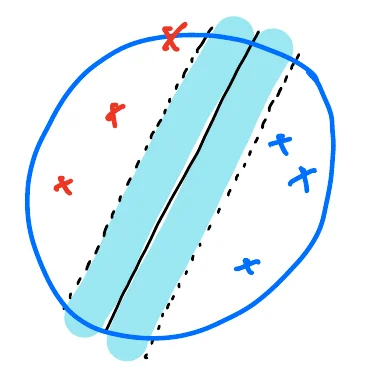
Theorem 16 (VC dimension of large margin hyperplanes)

Let $X_1,\dots ,X_n\in {\mathbb{R}}^d$ lie in a sphere of radius $R>0$ and let ${\mathcal{H}}_{\rho }$ be the linear classifiers with margin $\rho$, restricted to the sphere. Then

$$\mathrm{VC}({\mathcal{H}}_{\rho })=\min \left\{\frac{R^2}{{\rho }^2},d+1\right\}$$

Proof outline

We ask how large $n$ can be such that we can still shatter $n$ points with margin $\rho$ (never more than $d+1$). The most spread-out configuration of $n$ points in a ball of radius $R$ is a regular simplex with vertices on the sphere in ${\mathbb{R}}^{n-1}$: $\Vert x_i\Vert =R$, $⟨x_i,x_j⟩=-R^2/(n-1)$ (the slide writes $R^2/(n-1)$; for a simplex centred at the origin the inner products are negative). Split the points into $P$ (label $+1$) and $N$ (label $-1$); the distance between their convex hulls is the margin. By elementary but lengthy computations it is smallest when $P$ and $N$ have the same size, and then equals $R/\sqrt{n}$. Setting $\rho =R/\sqrt{n}$ and solving gives $n=R^2/{\rho }^2$. $\square$

Trap

Slide 62 states the margin result as $\min \{d,2R^2/{\rho }^2\}+1$, Theorem 16 on slide 73 as $\min \{R^2/{\rho }^2,d+1\}$. The constants differ; the message is the same: the margin bound does not depend on the dimension.

Discussion

The VC bound for general hyperplanes depends on the dimension, which is natural. The margin-based bound does not depend on $d$ at all, but it needs extra knowledge about the data distribution (a margin). We have seen the same ratio $R^2/{\rho }^2$ in the perceptron mistake bound (Lecture 2).

VC dimension of neural networks

Slides 77-86

VC dimension of a 2-layer network (sketch)

Input $x\in {\mathbb{R}}^d$, $N$ hidden units $f_i(x)=\mathrm{sign}(⟨w_i,x⟩+b_i)$, output $u(x)=\mathrm{sign}(⟨\tilde{w},(f_1(x),\dots ,f_N(x))⟩+b)$. Then the VC dimension is of order $O(Nd\log (Nd))$.

Proof sketch

Step 1: hypothesis classes. ${\mathcal{H}}_i$ = class of neuron $i$, ${\mathcal{H}}^{\prime }$ = class of the output unit; the network class is the composition $\mathcal{H}={\mathcal{H}}^{\prime }\circ ({\mathcal{H}}_1\times \cdots \times {\mathcal{H}}_N)$.

Step 2: individual classes. Each neuron is a linear classifier: $\mathrm{VC}({\mathcal{H}}_i)=d+1$, so $\mathcal{N}({\mathcal{H}}_i,n)\le n^{d+1}$. The output unit has $N$ inputs: $\mathrm{VC}({\mathcal{H}}^{\prime })=N+1$, $\mathcal{N}({\mathcal{H}}^{\prime },n)\le n^{N+1}$.

Step 3: combine. Shattering coefficients multiply under such compositions (a lemma, skipped): $\mathcal{N}(\mathcal{H},n)\le \mathcal{N}({\mathcal{H}}^{\prime },n)\cdot {\prod }_i\mathcal{N}({\mathcal{H}}_i,n)\le n^{N(d+1)+N+1}\approx n^{Nd}$.

Step 4: from the growth function to the VC dimension. The VC dimension is where the growth function stops being $2^n$. Solve $n^{Nd}<2^n$: with some work this gives $n\approx Nd\log (Nd)$. $\square$

• Typical results: a 2-layer network (threshold, sigmoid, ReLU activations) has VC dimension of order $O(W\log W)$ with $W$ the number of parameters, consistent with $W=Nd$ above. Multi-layer ReLU networks with $L$ layers: $O(LW\log W)$.
• Key technique in these proofs: counting regions. Fix a data point $x_1$; in the space of all parameter vectors $w$ (not the data space), the set where $x_1$ is classified positive is bounded by a separating curve. Adding points $x_2,x_3,\dots$ adds curves; each region corresponds to one labeling of the data. The number of regions is the number of labelings, and one has to be clever to count them.
• Discussion: the bound depends heavily on the dimension. Modern networks are very large, so VC generalization bounds are vacuous and cannot explain why neural networks learn (see Lecture 8).

Rademacher complexity

Slides 87-89

The shattering coefficient is a purely combinatorial object: it ignores the actual distribution. This seems suboptimal.

Rademacher complexity

Fix $n$ and let ${\sigma }_1,\dots ,{\sigma }_n$ be i.i.d. fair coin tosses with values $\pm 1$. The Rademacher complexity of $\mathcal{F}$ is

$${\mathrm{Rad}}_n(\mathcal{F}):=E\underset{f\in \mathcal{F}}{\sup }\frac{1}{n}\sum _{i=1}^n{\sigma }_{i}f(X_i)$$

with the expectation over the random points $X_i$ and the random labels ${\sigma }_i$. It measures how well the class can fit random labels.

Theorem 17 (Rademacher generalization bound)

With probability at least $1-\delta$, for all $f\in \mathcal{F}$,

$$R(f)\le R_n(f)+2{\mathrm{Rad}}_n(\mathcal{F})+\sqrt{\frac{\log (1/\delta )}{2n}}$$

(Proofs are beyond the scope of the lecture.) These bounds tend to be sharper than the combinatorial ones, and computing Rademacher complexities is in many cases much simpler than computing shattering coefficients or VC dimensions.

Mini example: two extreme classes

A single function $f_0$: $E\frac{1}{n}{\sum }_i{\sigma }_i{f}_0(X_i)=0$, so ${\mathrm{Rad}}_n=0$. All functions $\mathcal{X}\to \{\pm 1\}$ (with distinct points): choose $f(X_i)={\sigma }_i$, then the sum is $1$ and ${\mathrm{Rad}}_n=1$: the class fits any random labeling, and the bound is useless.

Generalization bounds: summary

Slide 90

The common form

With probability at least $1-\delta$, for all $f\in \mathcal{F}$:

$$R(f)\le R_n(f)+\text{capacity term}+\text{confidence term}$$

The capacity term measures the size of the function class, the confidence term how certain we are about the statement.

• Generalization bounds answer whether a learning algorithm is consistent within $\mathcal{F}$. They give insight but are not practical for concrete numbers.
• They concern the estimation error, not the approximation error.
• They are worst-case bounds: worst case over all distributions, and worst case over all learning algorithms that pick a function from $\mathcal{F}$.

Capacity measure	Bound on ${\sup }_f|R(f)-R_n(f)|$ (w.p. $1-\delta$)	Rate
fixed function	$\sqrt{\log (1/\delta )/(2n)}$	$1/\sqrt{n}$
$m$ functions	$\sqrt{(\log (2m)+\log (1/\delta ))/(2n)}$	$\sqrt{\log m/n}$
shattering coefficient	$2\sqrt{(\log \mathcal{N}(\mathcal{F},2n)-\log \delta )/n}$	needs $\log \mathcal{N}(\mathcal{F},2n)/n\to 0$
VC dimension $d$	$2\sqrt{(d\log (2en/d)-\log \delta )/n}$	$\sqrt{d\log n/n}$, $n\sim d/{\epsilon }^2$
Rademacher	$2{\mathrm{Rad}}_n(\mathcal{F})+\sqrt{\log (1/\delta )/(2n)}$	depends on $P$

Limitations and outlook

Limitations of SLT and the ERM principle

Slides 91-93

• The standard approach of SLT proves generalization by bounding the capacity of the function class. It revealed many important principles, and it applies primarily to the under-parameterized regime, where uniform convergence can be controlled.
• It is often technically challenging (how to compute the VC dimension or the Rademacher complexity of the class of a particular algorithm?).
• It gives worst-case guarantees over all functions in the class rather than looking at the actual algorithm. In particular, it does not matter which ERM minimizer an algorithm selects: the bounds apply to all of them or to none.
• In the overparameterized regime the bounds are still valid but vacuous. For linear classification with $d\gg n$ the bound just says $R(f)-R_n(f)<$ something large. Correct, but useless.

Different minima with different properties

Slides 94-95

Many empirical risk minimizers, some good and some bad

• Data in ${\mathbb{R}}^d$ from $N(0,I_d)$, true output $y=x^{(1)}$ (the first coordinate), i.e. $y=⟨w^{\ast },x⟩$ with $w^{\ast }=e_1=(1,0,\dots ,0)$. Minimize the squared loss on $n$ training points with $d\gg n$.
• The linear system $Y=Xw$ is under-determined, with many solutions: the true $w=e_1$ (test error 0), but also every $w=e_1+v$ with $v\in \ker (X)$. The test error of such a vector is $E(|⟨w^{\ast },x⟩-⟨w,x⟩{|}^2)=\Vert v{\Vert }^2$, as large as we want.
• VC theory gives nothing here (the bound is large when $d\gg n$). Some minimizers are good, some are bad. Observe for later: the good solution has the minimum norm among all solutions.

Outlook

Slide 96

In the overparameterized regime we need a mechanism that selects a good solution among the many minimizers. Principles that help:

• Stability: stable optima tend to generalize better (Lecture 4).
• Explicit regularization: reduce the capacity of the solution space; then standard bounds apply again in some cases (Lecture 5).
• Implicit regularization: some optimization algorithms such as SGD converge to the minimum norm solution; under favourable assumptions (benign overfitting) such solutions generalize (Lecture 8).

Task: VC dimension of two-sided half-lines

Exam-style task: a VC dimension with a bound (4 P)

$\mathcal{F}=\{1_{[a,\infty )}:a\in \mathbb{R}\}\cup \{1_{(-\infty ,a]}:a\in \mathbb{R}\}$: positive on a right or on a left half-line.

(a) (1 P, easy) Show that $\mathcal{N}(\mathcal{F},n)=2n$ for $n\ge 1$.

(b) (1.5 P, harder) Determine $\mathrm{VC}(\mathcal{F})$ and check the value $\mathcal{N}(\mathcal{F},n)$ against Sauer-Shelah.

(c) (1.5 P, transfer) Evaluate the capacity term $2\sqrt{(\log \mathcal{N}(\mathcal{F},2n)-\log \delta )/n}$ of Theorem 10 for $n=1000$ and $\delta =0.05$.

Solution

(a) On $x_1<\cdots <x_n$, right half-lines realize the $n+1$ labelings "$-\cdots -+\cdots +$" (a suffix positive), left half-lines the $n+1$ labelings with a positive prefix. All-positive and all-negative are counted twice: $2(n+1)-2=2n$. (1 P)

(b) $n=2$: $4=2^2$, shattered. $n=3$: $6<8$ ($(+,-,+)$ and $(-,+,-)$ are impossible). So $\mathrm{VC}=2$. Sauer-Shelah allows $1+n+\left(\genfrac{}{}{0ex}{}{n}{2}\right)$; indeed $2n\le 1+n+n(n-1)/2$ for all $n\ge 1$. (1.5 P)

(c) $\mathcal{N}(\mathcal{F},2000)=4000$: $\log 4000\approx 8.29$, $-\log 0.05\approx 3.00$, sum $11.29$, divided by 1000 gives $0.0113$, root $0.106$, times 2: $\approx 0.21$. So with probability $0.95$ every $f\in \mathcal{F}$ has $R(f)\le R_n(f)+0.21$. (1.5 P)

Self-Test

Question cards (14)

Distinguish consistency w.r.t. $\mathcal{F}$, Bayes consistency and universal consistency.

Answer

W.r.t. $\mathcal{F}$ and $P$: $R(f_n)\to R(f_{\mathcal{F}})$ in probability (estimation error only). Bayes-consistent: $R(f_n)\to R(f^{\ast })$. Universally: the respective property holds for all $P$.

State Hoeffding's inequality with its assumptions.

Answer

For independent $Z_1,\dots ,Z_n\in [0,1]$: $P(|S_n-E(S_n)|\ge \epsilon )\le 2\exp (-2n{\epsilon }^2)$. Identical distributions are not needed; independence and the bounded range are.

State McDiarmid's inequality and derive Hoeffding from it.

Answer

If changing the $i$-th argument changes $f$ by at most $c_i$ and the $X_i$ are independent: $P(|f-Ef|\ge \epsilon )\le 2\exp (-2{\epsilon }^2/\sum c_i^2)$. For the mean of $[0,1]$ variables $c_i=1/n$, $\sum c_i^2=1/n$, giving $2\exp (-2n{\epsilon }^2)$.

How many test points do you need to estimate the error of a fixed classifier up to $\epsilon$, and why?

Answer

Of the order $1/{\epsilon }^2$: from $\delta =\exp (-2n{\epsilon }^2)$, $\epsilon =\sqrt{\log (1/\delta )/(2n)}$. For $\epsilon =1\%$ about $10,000$ points.

Define uniform convergence and show that it implies consistency of ERM.

Answer

$\forall \epsilon :P({\sup }_f|R_n(f)-R(f)|>\epsilon )\to 0$. Then $R(f_n)-R(f_{\mathcal{F}})\le (R(f_n)-R_n(f_n))+(R_n(f_{\mathcal{F}})-R(f_{\mathcal{F}}))\le 2{\sup }_f|R-R_n|$, since $R_n(f_n)\le R_n(f_{\mathcal{F}})$.

What does Theorem 7 (Vapnik and Chervonenkis 1971) add?

Answer

Uniform convergence is not only sufficient but also necessary: ERM is uniformly consistent w.r.t. $\mathcal{F}$ iff uniform convergence holds.

Derive the generalization bound for a finite class.

Answer

Union bound over the $m$ functions with Hoeffding: $P({\sup }_f|R-R_n|\ge \epsilon )\le 2m{e}^{-2n{\epsilon }^2}$. Set this to $\delta$: with probability $1-\delta$, $R(f)\le R_n(f)+\sqrt{(\log 2m+\log 1/\delta )/(2n)}$ for all $f$.

How should the number of cells $k$ of a partitioning estimator grow with $n$?

Answer

$k(n)/n\to 0$ for consistency w.r.t. ${\mathcal{F}}_{k(n)}$ (enough points per cell), and $k\to \infty$ for Bayes consistency (fine cells). In $d$ dimensions the error term is $k^d/n$: exponentially many samples.

Define the shattering coefficient and explain the idea of symmetrization.

Answer

$\mathcal{N}(\mathcal{F},n)={\max }_{X_1..X_n}|{\mathcal{F}}_{X_1,\dots ,X_n}|$, the maximal number of labelings. Symmetrization replaces $R$ by the risk on a ghost sample; then only the values on $2n$ points matter, so the supremum runs over at most $\mathcal{N}(\mathcal{F},2n)$ functions and the finite-class bound applies.

Define shattering and the VC dimension. What do you have to show for $\mathrm{VC}=d$?

Answer

$\mathcal{F}$ shatters $X_1..X_n$ if it realizes all $2^n$ labelings. $\mathrm{VC}$ is the largest $n$ for which some $n$-point set is shattered. For $\mathrm{VC}=d$: one set of $d$ points is shattered, and no set of $d+1$ points is.

State the Sauer-Shelah lemma and the dichotomy it implies.

Answer

For VC dimension $d$: $\mathcal{N}(\mathcal{F},n)\le {\sum }_{i=0}^d\left(\genfrac{}{}{0ex}{}{n}{i}\right)\le (en/d{)}^d$ for $n\ge d$. So the growth function is either $2^n$ for all $n$ (VC $=\infty$) or polynomial of degree $d$; nothing in between.

Prove that linear classifiers in ${\mathbb{R}}^d$ have VC dimension $d+1$.

Answer

Shatter $0,e_1,\dots ,e_d$ with $b=y_0$, $w_i=y_i-b$. For $d+2$ points, Radon’s theorem gives a partition into $P,N$ with intersecting convex hulls; labeling $P$ positive and $N$ negative cannot be realized.

What is the VC dimension of margin classifiers, and why is it interesting?

Answer

For data in a ball of radius $R$ and margin $\rho$: $\min \{R^2/{\rho }^2,d+1\}$. It does not depend on the dimension, but it needs the assumption that the data has a margin.

Why are VC bounds useless in the overparameterized regime? Give the example of the lecture.

Answer

With $d\gg n$ the capacity term is large, so the bound is vacuous. Least squares with $y=x^{(1)}$: all $w=e_1+v$, $v\in \ker X$, interpolate the data, but the test error is $\Vert v{\Vert }^2$. The bound cannot tell good from bad minimizers; the good one has minimum norm.

Multiple Choice

Multiple choice (8)

Which assumption of Hoeffding's inequality is essential?

• the $Z_i$ are identically distributed

• the $Z_i$ are independent and take values in a bounded interval

• the $Z_i$ are Gaussian

• $n\ge 30$

Explanation

Slide 12: the variables need not have the same distribution, as long as the range is controlled; independence is crucial.

For a finite class of $m$ functions, the capacity term of the generalization bound grows with $m$ like

• $m$

• $\sqrt{m}$

• $\sqrt{\log m}$

• $m\log m$

Explanation

The union bound puts $m$ into the failure probability $2m{e}^{-2n{\epsilon }^2}$; solving for $\epsilon$ gives $\sqrt{(\log 2m+\log (1/\delta ))/(2n)}$.

A class has $N(\mathcal{F},1)=2$, $N(\mathcal{F},2)=4$, $N(\mathcal{F},3)=6$. Which statement is true?

• $\mathrm{VC}(\mathcal{F})=3$

• $N(\mathcal{F},10)$ can be $2^{10}$

• $\mathrm{VC}(\mathcal{F})=2$ and $N(\mathcal{F},10)\le 56$

• the VC dimension cannot be determined without knowing the points

Explanation

The last shattered size is 2 ($4=2^2$, $6<8$). Once a size is not shattered, no larger one is, and Sauer-Shelah gives $1+10+45=56$. The growth function is a maximum over all point sets, so it does not depend on particular points.

The VC dimension of linear classifiers $\mathrm{sign}(⟨w,x⟩+b)$ on ${\mathbb{R}}^d$ is

• $d$

• $d+1$

• $2d$

• $\infty$

Explanation

Proposition 15. Without the offset $b$ it would be $d$.

Which statement about proving a VC dimension is true?

• A class with $m$ real parameters has VC dimension $m$.

• To show $\mathrm{VC}(\mathcal{F})\ge 3$, you must show that every set of 3 points is shattered.

• To show $\mathrm{VC}(\mathcal{F})\le 2$, you must show that no set of 3 points is shattered.

• A class with VC dimension 2 realizes at most 3 labelings of any 3 points.

Explanation

The lower bound needs one shattered set, the upper bound needs “no set”. Parameters are not the VC dimension ($\mathrm{sgn}\sin (tx)$ has one parameter and VC $=\infty$). With VC 2, up to $1+3+3=7$ labelings of 3 points are possible (intervals realize 7).

According to the VC bound, how many samples are needed (up to logarithmic factors) for accuracy $\epsilon$ with a class of VC dimension $d$?

• $d/\epsilon$

• $d/{\epsilon }^2$

• $2^d/{\epsilon }^2$

• $\log (d)/{\epsilon }^2$

Explanation

The capacity term is $\approx \sqrt{d\log n/n}$; setting it to $\epsilon$ gives $n\approx d/{\epsilon }^2$ (slide 67).

What does the Rademacher complexity of a class measure?

• the number of parameters of the class

• the largest set of points the class shatters

• how well the class can fit random $\pm 1$ labels, in expectation over the data

• the approximation error of the class

Explanation

${\mathrm{Rad}}_n=E{\sup }_f\frac{1}{n}{\sum }_i{\sigma }_{i}f(X_i)$ with random signs; unlike the VC dimension, it depends on the distribution of the $X_i$.

Which statement about generalization bounds is true?

• They bound the approximation error of a class.

• They depend on which ERM minimizer the algorithm picks.

• They are worst case over distributions and over all functions in the class.

• They give tight numbers for deep networks.

Explanation

Slide 90: they concern the estimation error and hold uniformly over $\mathcal{F}$, which is why they cannot distinguish good from bad minimizers and are vacuous for large networks.

References

All sources cited on the slides, in slide order (11 entries)

Slide	Source	Key point
4	von Luxburg and Schölkopf, “Statistical Learning Theory: Models, Concepts, and Results”, 2011	high-level overview
4	Bousquet, Boucheron and Lugosi, “Introduction to Statistical Learning Theory”, 2003	more technical introduction
4	Devroye, Györfi and Lugosi, A Probabilistic Theory of Pattern Recognition, Springer 1996	the classical book
4	Shalev-Shwartz and Ben-David (online); Bach, Learning Theory from First Principles	general textbooks
8	Bach, Sec. 1.2	concentration inequalities
8	McDiarmid, “On the Method of Bounded Differences”, Surveys in Combinatorics, 1989	McDiarmid’s inequality
8	Boucheron, Lugosi and Massart, Concentration Inequalities	details on concentration
11	Chernoff 1952; Hoeffding 1963	Hoeffding’s inequality
26	Vapnik and Chervonenkis, 1971	uniform convergence is necessary and sufficient
63	Vapnik, Chervonenkis; Sauer; Shelah	Sauer-Shelah lemma
68	Hush and Scovel, “On the VC Dimension of Bounded Margin Classifiers”, Machine Learning, 2001	VC dimension with a margin

Related

• Previous: Lecture 2: Perceptron Mistake Bound · Next: Lecture 4: Algorithmic Stability · Course: Overview
• Concepts: Hoeffding Inequality, Uniform Convergence, Generalization Bound, Shattering Coefficient, VC Dimension, Rademacher Complexity, Consistency, Margin
• Exercises: Sheet 3, Exercises 1-2 (Hoeffding, validating many classifiers); Sheet 4, Exercises 2-3 (VC dimension, one-vs-all bounds)