Lecture 2: Perceptron Mistake Bound

TL;DR

1. Linear classifier without offset: $f(x)=\mathrm{sign}(⟨w,x⟩)$. A point is classified correctly iff $y_i⟨w,x_i⟩>0$.
2. Perceptron: start at $w_0=0$; whenever $y_t⟨w_{t-1},x_t⟩\le 0$ (a mistake), update $w_t=w_{t-1}+y_t{x}_t$. This is SGD with step size 1 on the linear loss $\max \{0,-y⟨w,x⟩\}$.
3. The distance of $x$ to the hyperplane $H_w$ is $y⟨w,x⟩/\Vert w\Vert$ (signed with the label); the margin is the smallest distance of a training point: $\rho ={\min }_i{y}_i⟨w,x_i⟩/\Vert w\Vert$.
4. Theorem 1 (Novikoff 1962): if $\Vert x_i\Vert \le R$ and some $w^{\ast }$ separates the data with margin $\rho >0$, the perceptron makes at most $R^2/{\rho }^2$ mistakes. The bound does not depend on the dimension.
5. Theorem 2: trained until 0 training errors, the perceptron’s test error is at most $\frac{1}{n+1}E(R^2/{\rho }^2)$: a fast rate $1/n$, again dimension-free. The proof uses the leave-one-out principle, an early form of stability.
6. Without separability there is no convergence; with the hinge-type slack $D$ one gets $M\le (R+D{)}^2/{\rho }^2$ (Freund and Schapire 1999).

Exam relevance

• Mock exam, task 1 (2 P): run the perceptron by hand on three points in ${\mathbb{R}}^2$ without offset, starting at $w=(0,0)$, sweeping until a full sweep makes no update, counting $y_i⟨w,x_i⟩\le 0$ as a mistake, and filling in a worksheet. Train it with the task below and the widget.
• Computations: distance to a hyperplane, margin of a given $w$, the mistake bound $R^2/{\rho }^2$, the generalization bound for given $R$, $\rho$, $n$.
• Multiple choice: what the bound depends on (not on $d$), which loss the perceptron minimizes, rate $1/n$, the role of the learning rate.
• Sheet 4, Exercise 1: margin perceptron (updates while $y_i⟨w,x_i⟩<{\rho }_0$, bound $(R^2+2{\rho }_0)/{\rho }^2$).

Overview: 1. The perceptron algorithm, 2. The perceptron minimizes the linear loss by SGD, 3. Margin and the mistake bound, 4. Generalization error of the perceptron, 5. Outlook: the non-separable case.

The perceptron algorithm

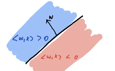
Linear classification

Slides 3-5

(Literature: Hardt and Recht Sec. 3, Mohri Sec. 7.1, Shalev-Shwartz and Ben-David Sec. 21.4.) This lecture is a warmup: a first, simple example of how one can prove that a learning algorithm works.

Linear classifier without offset

Training points $x_1,x_2,\cdots \in {\mathbb{R}}^d$ with labels $y_1,y_2,\cdots \in \{\pm 1\}$. We study

$$f(x)=\mathrm{sign}(⟨w,x⟩),w\in {\mathbb{R}}^d$$

without an offset parameter $b$: the separating hyperplane $H_w=\{x:⟨w,x⟩=0\}$ passes through the origin.

Correct classification

A point $(x_i,y_i)$ is classified correctly $⟺y_i⟨w,x_i⟩>0$.

Slide 5: w is the normal vector of the hyperplane; ⟨w, x⟩ > 0 on the side it points to.

The perceptron algorithm

Slide 6

Require: (x_1, y_1), ..., (x_n, y_n)
 1: w_0 ← 0
 2: t ← 1
 3: N ← n
 4: while t ≤ N do
 5:     if y_t ⟨w_{t-1}, x_t⟩ ≤ 0 then     ▷ x_t is wrongly classified
 6:         w_t ← w_{t-1} + y_t x_t          ▷ update w
 7:     else                                  ▷ x_t is correctly classified
 8:         w_t ← w_{t-1}                     ▷ keep current w
 9:     end if
10:     t ← t + 1
11: end while

As written, the algorithm makes one pass through the $n$ points. To reach 0 training errors, one cycles through the data again and again until a full pass (a “sweep”) makes no update. This is the version used in the mistake bound and in the exam.

Ties count as mistakes

The condition is $y_t⟨w,x_t⟩\le 0$, with "$\le$". At the start $w_0=0$, so $y⟨w_0,x⟩=0$: the first point always triggers an update. With "$<$" the algorithm would never leave $w=0$.

Run the perceptron step by step, one sweep at a time or until convergence. The log on the right is the worksheet of the exam task. Click in the plane to add your own points. The cards show R, the best margin ρ of any line through the origin and the bound R²/ρ².

Task: the perceptron by hand

Exam-style task: the perceptron by hand (4 P)

Points in ${\mathbb{R}}^2$, no offset: $x_1=(1,0)$ with $y_1=+1$, $x_2=(1,1)$ with $y_2=-1$, $x_3=(0,1)$ with $y_3=-1$. Start with $w=(0,0)$, sweep in the order $x_1,x_2,x_3$ and repeat until a full sweep makes no update. Count $y_i⟨w,x_i⟩\le 0$ as a mistake; on a mistake set $w\leftarrow w+y_i{x}_i$.

(a) (2 P, easy) Carry out the run: for each step give $y_i⟨w,x_i⟩$, whether it is a mistake, and $w$ afterwards.

(b) (1 P, harder) $w^{\ast }=(1,-2)$ separates the data. Compute $R$, the margin $\rho$ of $w^{\ast }$ and the mistake bound. Is your run consistent with it?

(c) (1 P, transfer) Run the update $w\leftarrow w+\eta y_i{x}_i$ with $\eta =2$ instead. How many mistakes are made, and what is the final $w$?

Solution

(a) (2 P: 1 P for the first two sweeps, 1 P for sweeps 3 and 4 and the stop)

sweep	point	$y_i⟨w,x_i⟩$	mistake?	$w$ after
1	$x_1$	$0$	yes	$(1,0)$
1	$x_2$	$-1$	yes	$(0,-1)$
1	$x_3$	$1$	no	$(0,-1)$
2	$x_1$	$0$	yes	$(1,-1)$
2	$x_2$	$0$	yes	$(0,-2)$
2	$x_3$	$2$	no	$(0,-2)$
3	$x_1$	$0$	yes	$(1,-2)$
3	$x_2$	$1$	no	$(1,-2)$
3	$x_3$	$2$	no	$(1,-2)$
4	all	$1,1,2$	no	stop

5 mistakes, final $w=(1,-2)$. Watch the ties: in sweeps 2 and 3, $y⟨w,x⟩=0$ counts as a mistake.

(b) $R={\max }_i\Vert x_i\Vert =\Vert (1,1)\Vert =\sqrt{2}$. With $\Vert w^{\ast }\Vert =\sqrt{5}$: $y_i⟨w^{\ast },x_i⟩=1,1,2$, so $\rho =1/\sqrt{5}$. Bound $R^2/{\rho }^2=2\cdot 5=10\ge 5$ ✓. (1 P)

(c) With $w_0=0$, every $w_t$ is exactly $\eta$ times the $w_t$ of the run with $\eta =1$, so all signs $y_i⟨w,x_i⟩$ are the same: again 5 mistakes, final $w=(2,-4)$. The learning rate does not matter for the perceptron started at 0. (1 P)

Perceptron performs linear loss minimization

The linear loss

Slides 7-9

0-1 loss and linear loss

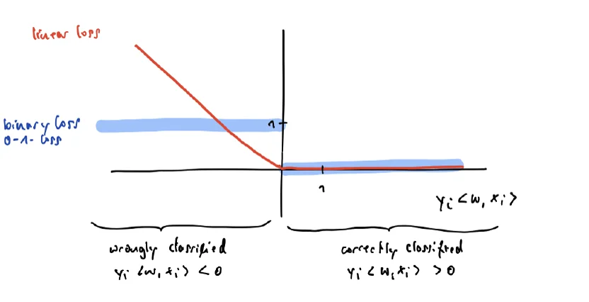
The “natural” loss for classification is the 0-1 loss: $\ell (⟨w,x_i⟩,y_i)=0$ if $f(x_i)=y_i$ and 1 otherwise. To quantify “how wrong” the function is, one can use the linear loss

$$\ell (⟨w,x_i⟩,y_i)=\max \{0,-y_i⟨w,x_i⟩\}$$

Slide 9: the linear loss is 0 on correctly classified points and grows linearly with how far a point is on the wrong side.

Linear loss minimization by SGD

Slides 10-12

Goal: find the linear classifier that minimizes the empirical risk

$$\underset{w}{\min }\frac{1}{n}\sum _{i=1}^n\ell (y_i⟨w,x_i⟩)$$

with the linear loss. How would we solve this, and how is it related to the perceptron?

Gradient descent and stochastic gradient descent

Minimize $R_n(w)=\frac{1}{n}{\sum }_{i=1}^n\ell (y_i,f_w(x_i))$ over $w\in {\mathbb{R}}^d$ (loss differentiable in $w$).

• Gradient descent: start with some $w_0$, compute ${\nabla }_w{R}_n(w)=\frac{1}{n}{\sum }_i{\nabla }_w\ell (y_i,f_w(x_i))$, update $w_{t+1}=w_t-\eta {\nabla }_w{R}_n(w_t)$ with step size (learning rate) $\eta$.
• Stochastic gradient descent (SGD): start with some $w_0$, pick a random $i$, compute only ${\nabla }_w\ell (y_i,f_w(x_i))$ and update $w_{t+1}=w_t-\eta {\nabla }_w\ell (y_i,f_w(x_i))$.

Perceptron runs SGD with the linear loss

Slides 13-14

Gradient of the linear loss

$$\ell (⟨w,x_i⟩,y_i)=\{\begin{array}{ll}0& \text{if }-y_i⟨w,x_i⟩<0\\ -y_i⟨w,x_i⟩& \text{otherwise}\end{array}$$ $${\nabla }_w\ell =\{\begin{array}{ll}0& \text{if }-y_i⟨w,x_i⟩<0\\ -y_i{x}_i& \text{otherwise}\end{array}$$

An SGD step with $\eta =1$ is $w\leftarrow w-(-y_i{x}_i)=w+y_i{x}_i$ on a mistake and no change otherwise: exactly the perceptron update.

So the perceptron performs a simplified version of SGD (step size $\eta =1$, one pass through the training points, in order). At $y_i⟨w,x_i⟩=0$ the loss has a kink; the case “otherwise” takes $-y_i{x}_i$ there, which is why ties trigger an update.

By itself this doesn’t mean a lot. Two questions remain: (1) does it really converge to an ERM classifier that minimizes the training loss? (2) what about the test error?

Mistake bound for the perceptron

Distance of a point to a hyperplane

Slides 15-17

We want to prove: if the training points are “well separable”, the number of updates needed to find a classifier with 0 training error is bounded. First we make “well separable” precise.

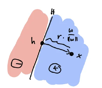
Distance to the hyperplane

Let $H$ be the hyperplane with normal vector $w$, $x$ a point with $⟨w,x⟩>0$, $h\in H$ the closest point to $x$ and $r$ the distance. Then $x=h+r\cdot \frac{w}{\Vert w\Vert }$, and since $⟨h,w⟩=0$:

$$⟨x,w⟩=⟨h,w⟩+r\frac{⟨w,w⟩}{\Vert w\Vert }=r\Vert w\Vert \Rightarrow r=\frac{⟨x,w⟩}{\Vert w\Vert }$$

If $⟨x,w⟩<0$, then $r=-\frac{⟨x,w⟩}{\Vert w\Vert }$. For a correctly classified labeled point both cases are

$$r=y\frac{⟨x,w⟩}{\Vert w\Vert }$$

Slide 17: x = h + r · w/‖w‖.

The margin of a separating hyperplane

Slide 18

Margin

For training points $(x_1,y_1),\dots ,(x_n,y_n)$ and a linear classifier $⟨w,x⟩$ that separates them, the margin is the smallest distance of a training point to the hyperplane $H_w$:

$$\rho =\underset{i}{\min }\mathrm{distance}(x_i,H_w)=\underset{i=1,\dots ,n}{\min }\frac{y_i⟨w,x_i⟩}{\Vert w\Vert }$$

Mini example

$w=(3,4)$, $\Vert w\Vert =5$. The point $x=(1,2)$ with $y=+1$ has distance $(3+8)/5=2.2$. The point $x^{\prime }=(1,-1)$ with $y^{\prime }=-1$ has distance $-(3-4)/5=0.2$. The margin of $w$ on these two points is $0.2$. Scaling $w$ does not change distances or the margin.

Theorem 1: the perceptron mistake bound

Slides 19-23

Theorem 1 (perceptron mistake bound, Novikoff 1962)

Let $\{(x_i,y_i){\}}_{i=1}^N$ with $\Vert x_i\Vert \le R$ for all $i$. Assume there is a separating hyperplane induced by $w^{\ast }\in {\mathbb{R}}^d$ with margin $\rho >0$ on the training points. Then the number of mistakes of the perceptron is at most

$$\frac{R^2}{{\rho }^2}$$

In particular, after at most $R^2/{\rho }^2$ updates the perceptron has found a linear classifier with 0 training errors.

Intuition

Every mistake pushes $w$ a bit towards $w^{\ast }$ (the projection onto $w^{\ast }$ grows by at least $\rho$), but the length of $w$ grows slowly (its square by at most $R^2$). After $M$ mistakes the projection is $\ge M\rho$ while the length is $\le \sqrt{M}R$. A projection can never be longer than the vector, so $M\rho \le \sqrt{M}R$, i.e. $M\le R^2/{\rho }^2$.

Proof of Theorem 1

Step 1: upper bound on $\Vert w\Vert$. Suppose the algorithm misclassifies $x_t$, so $y_t⟨w_t,x_t⟩\le 0$. With the update rule and $y_t^2=1$:

$$\Vert w_{t+1}{\Vert }^2=\Vert w_t+y_t{x}_t{\Vert }^2=\Vert w_t{\Vert }^2+2y_t⟨w_t,x_t⟩+\Vert x_t{\Vert }^2\le \Vert w_t{\Vert }^2+R^2(\star )$$

Let $I$ be the indices where a mistake happened and $M=|I|$. Summing $(\star )$ over $I$: ${\sum }_{i\in I}(\Vert w_{i+1}{\Vert }^2-\Vert w_i{\Vert }^2)\le M{R}^2$. Without a mistake there is no update, so the sum can be taken over all steps, and it telescopes to $\Vert w_n{\Vert }^2-\Vert w_0{\Vert }^2=\Vert w_n{\Vert }^2$:

$$\Vert w_n{\Vert }^2\le M{R}^2(\star \star )$$

Step 2: lower bound on $\Vert w\Vert$. By the margin assumption, $\rho \le y_i⟨w^{\ast },x_i⟩/\Vert w^{\ast }\Vert$ for all $i$. Summing over the mistakes and using Cauchy-Schwarz:

$$M\rho \le \sum _{i\in I}\frac{y_i⟨w^{\ast },x_i⟩}{\Vert w^{\ast }\Vert }=\frac{1}{\Vert w^{\ast }\Vert }⟨w^{\ast },\sum _{i\in I}{y}_i{x}_i⟩\le \Vert \sum _{i\in I}{y}_i{x}_i\Vert =\Vert \sum _i(w_{i+1}-w_i)\Vert =\Vert w_n\Vert (\#)$$

(for mistakes $w_{i+1}=w_i+y_i{x}_i$, then the telescoping sum again).

Step 3: combine. $(\star \star )$ and $(\#)$ give $M^2{\rho }^2\le \Vert w_n{\Vert }^2\le M{R}^2$, so $M\le R^2/{\rho }^2$. $\square$

Trap

On slide 20 the condition used in step 1 is written as "$⟨w_t,x_t⟩\le 0$". What the proof needs is the mistake condition $y_t⟨w_t,x_t⟩\le 0$, which makes the cross term $2y_t⟨w_t,x_t⟩$ non-positive.

Discussing the bound

Slide 24

• The bound does not depend on the dimension $d$.
• Implicit in the proof: SGD does not pick just any ERM minimizer, it picks a special one with nice guarantees. This is implicit regularization of SGD, which comes back in Lecture 8.
• The bound only holds under the assumption on the data (a margin). Margins pop up in many places in ML: SVMs, boosting (Lecture 6).
• The theorem only covers the separable case. In the non-separable case (or with margin 0) no bound exists.
• Learning rate $\eta$ in $w_{t+1}=w_t+\eta y_t{x}_t$: see the assignment (and part (c) of the task above).
• The bound only considers training errors. What about generalization?

Task: margin and mistake bound

Exam-style task: margin and mistake bound (4 P)

Training data: $x_1=(3,1)$ and $x_2=(1,2)$ with label $+1$, $x_3=(-1,-1)$ and $x_4=(0,-2)$ with label $-1$. Two candidate normal vectors: $w_A=(1,1)$ and $w_B=(1,2)$.

(a) (1 P, easy) Compute the margin of $w_A$ and of $w_B$ on the data.

(b) (1.5 P, harder) Compute $R$ and the best mistake bound you can derive from $w_A$ or $w_B$.

(c) (1.5 P, transfer) A new point $x_5=(4,-3)$ with label $+1$ is added. Is the data still separated by $w_A$? What happens to the bound, and why can a single point make it much worse?

Solution

(a) $w_A$, $\Vert w_A\Vert =\sqrt{2}$: $y_i⟨w_A,x_i⟩=4,3,2,2$, so ${\rho }_A=2/\sqrt{2}=\sqrt{2}\approx 1.41$. $w_B$, $\Vert w_B\Vert =\sqrt{5}$: $5,5,3,4$, so ${\rho }_B=3/\sqrt{5}\approx 1.34$. (1 P)

(b) $R=\max \Vert x_i\Vert =\Vert (3,1)\Vert =\sqrt{10}$. The larger margin gives the better bound: $R^2/{\rho }_A^2=10/2=5$ mistakes. (With $w_B$: $10/1.8\approx 5.6$.) (1.5 P)

(c) $⟨w_A,x_5⟩=1>0$: still separated, but the distance is only $1/\sqrt{2}\approx 0.71$, so ${\rho }_A$ drops to $0.71$. Also $R$ grows to $\Vert x_5\Vert =5$. The bound becomes $25/0.5=50$. The bound depends on the worst point twice: through the largest norm and through the smallest distance. (1.5 P)

Generalization error of the perceptron

Assumption: the distribution is linearly separable

Slides 25-26

To prove a generalization bound we make a strong assumption:

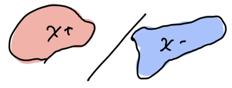
1. A deterministic function $f^{\ast }:\mathcal{X}\to \mathcal{Y}$ produces the true labels, $y=f^{\ast }(x)$.
2. The sets ${\mathcal{X}}^{+}=\{x:f^{\ast }(x)=+1\}$ and ${\mathcal{X}}^{-}=\{x:f^{\ast }(x)=-1\}$ are linearly separable: some hyperplane with parameters $w^{\ast }$ has them on different sides.

Slide 26: the positive and negative regions of the input space are linearly separable.

Theorem 2: bounding the test error

Slide 27

Theorem 2 (generalization error of the perceptron)

Let $P$ on $\mathcal{X}\times \mathcal{Y}$ be perfectly separable by a hyperplane and $S_{n+1}=\{(x_1,y_1),\dots ,(x_{n+1},y_{n+1})\}$ i.i.d. from $P$. Let $w(S_n)$ be the perceptron trained on $S_n=\{(x_1,y_1),\dots ,(x_n,y_n)\}$ until it makes no mistakes on $S_n$. Let $R(S_{n+1})$ be the radius of the ball containing all points of $S_{n+1}$, and $\rho (S_{n+1})$ the largest margin any hyperplane achieves on $S_{n+1}$. Then the probability that the classifier trained on $S_n$ errs on the new point is

$$P(y_{n+1}⟨w(S_n),x_{n+1}⟩<0)\le \frac{1}{n+1}E\left(\frac{R^2(S_{n+1})}{{\rho }^2(S_{n+1})}\right)$$

Discussion: scaling with $d$ and $n$

Slides 28-29

• The generalization error does not depend on the dimension of the space. That is cool.
• Suppose the distribution lives in a ball of radius $R^{\ast }$ and a hyperplane separates all points of $\mathcal{X}$ with margin ${\rho }^{\ast }$. Then for all sets $S_{n+1}$: $R(S_{n+1})\le R^{\ast }$ and $\rho (S_{n+1})\ge {\rho }^{\ast }$, so

Fast rate

$$P(\text{error})\le \frac{1}{n+1}E\left(\frac{R^2(S_{n+1})}{{\rho }^2(S_{n+1})}\right)\le \frac{1}{n+1}\frac{R^{\ast 2}}{{\rho }^{\ast 2}}$$

The generalization error (0-1 loss) decreases with rate $1/n$. In learning theory this is called a fast rate. (Typical rates in Lecture 3 are $1/\sqrt{n}$.)

Trap

Slide 29 writes the ratio without squares, $R/\rho$. Theorem 2 has $R^2/{\rho }^2$; the squares matter in computations (halving the margin quadruples the bound).

Proof: the leave-one-out argument

Slides 30-33

Proof of Theorem 2

Idea: leave-one-out. Consider the augmented sample $S_{n+1}=Z_1,\dots ,Z_n,Z_{n+1}$ with $Z_1,\dots ,Z_n$ for training and $Z_{n+1}$ for testing, and the leave-one-out sets $S^{-k}=Z_1,\dots ,Z_{k-1},Z_{k+1},\dots ,Z_{n+1}$. Since the data is i.i.d., it makes no difference (in expectation) whether we train on $S_n$ and test on $Z_{n+1}$, or train on $S^{-k}$ and test on $Z_k$. Let $w(S^{-k})$ be the weight vector after training on $S^{-k}$ to error 0.

Step 1.

$$\begin{array}{rl}P(y_{n+1}⟨w(S_n),x_{n+1}⟩<0)& =E(1\{y_{n+1}⟨w(S_n),x_{n+1}⟩<0\})\\ & =\frac{1}{n+1}\sum _{k=1}^{n+1}E(1\{y_k⟨w(S^{-k}),x_k⟩<0\})\\ & =\frac{1}{n+1}E(\sum _{k=1}^{n+1}1\{y_k⟨w(S^{-k}),x_k⟩<0\})(\star )\end{array}$$

(the same expectation for every $S^{-k}$).

Step 2: the sum. Run the perceptron on the whole sequence $Z_1,\dots ,Z_{n+1}$ from scratch. By the mistake bound it makes $M(S_{n+1})\le R^2(S_{n+1})/{\rho }^2(S_{n+1})$ mistakes, at the indices $J_{n+1}=\{i_1,\dots ,i_M\}$ (over all its cycles). If $k\notin J_{n+1}$, the point $Z_k$ never triggered an update, so removing it does not change the run: $w(S^{-k})$ equals the final vector on $S_{n+1}$, which classifies $Z_k$ correctly. So only indices in $J_{n+1}$ can contribute:

$$\sum _{k=1}^{n+1}1\{y_k⟨w(S^{-k}),x_k⟩<0\}\le \sum _{k\in J_{n+1}}1=|J_{n+1}|=M(S_{n+1})$$

Step 3. Plugging into $(\star )$:

$$(\star )\le \frac{1}{n+1}E(M(S_{n+1}))\le \frac{1}{n+1}E\left(\frac{R^2(S_{n+1})}{{\rho }^2(S_{n+1})}\right)\square$$

The leave-one-out principle and stability

Slides 34-35

Leave-one-out principle

The average leave-one-out error on a sample of size $n+1$ is an unbiased estimate of the average generalization error for samples of size $n$. (Proof: Holin p. 69/70, Lemma 4.1.)

The proof technique also hints at a principle we discuss in detail later: stability (Lecture 4). Stability asks how much the result of a learning algorithm changes if we remove one training point or replace it by a different one. With this technique one can prove very strong generalization bounds.

Task: the generalization bound

Exam-style task: generalization bound (4 P)

The data lies in a ball of radius $R^{\ast }=2$, and a hyperplane separates the whole input space with margin ${\rho }^{\ast }=0.5$. The perceptron is trained on $n$ points until it makes no training errors.

(a) (1 P, easy) Bound the test error for $n=999$.

(b) (1.5 P, harder) How many training points guarantee a test error of at most $0.5\%$?

(c) (1.5 P, transfer) The same problem is embedded in ${\mathbb{R}}^{1000}$ instead of ${\mathbb{R}}^{10}$ (extra coordinates are 0), and separately the margin is halved. How do the answers of (b) change?

Solution

(a) $\frac{1}{n+1}\frac{R^{\ast 2}}{{\rho }^{\ast 2}}=\frac{1}{1000}\cdot \frac{4}{0.25}=0.016$, i.e. $1.6\%$. (1 P)

(b) $\frac{16}{n+1}\le 0.005⟺n+1\ge 3200⟺n\ge 3199$. (1.5 P)

(c) The dimension does not appear in the bound: still $n\ge 3199$. Halving the margin multiplies $R^2/{\rho }^2$ by 4, so one needs $n+1\ge 12800$, i.e. $n\ge 12799$. (1.5 P)

Outlook: what if the data is not linearly separable?

Slide 36

Then one can prove more general versions of the theorem.

Mistake bound in the non-separable case (Freund and Schapire 1999)

Given a margin $\rho$, define the hinge-type loss of a point $(x,y)$ and the total slack

$$\delta (x,\rho ):=\max \{0,\rho -y⟨w,x⟩\},D:=(\sum _{i=1}^n\delta (x_i,\rho {)}^2{)}^{1/2}$$

Then the number of updates of the perceptron is bounded by

$$M\le \frac{(R+D{)}^2}{{\rho }^2}$$

(proof in the Mohri book). The generalization bound in this case is more complicated and only scales as $1/\sqrt{n}$.

For separable data with margin $\rho$ under $w$, all $\delta =0$, so $D=0$ and the bound is Theorem 1 again.

Summary

Result	Statement	Depends on
Perceptron update	on $y⟨w,x⟩\le 0$: $w\leftarrow w+yx$	SGD, $\eta =1$, linear loss
Distance, margin	$r=y⟨w,x⟩/\Vert w\Vert$, $\rho ={\min }_i{r}_i$	invariant to scaling $w$
Theorem 1 (mistake bound)	$M\le R^2/{\rho }^2$	$R$ and $\rho$, not $d$ or $n$
Theorem 2 (test error)	$\le \frac{1}{n+1}E(R^2/{\rho }^2)$	rate $1/n$, dimension-free
Non-separable	$M\le (R+D{)}^2/{\rho }^2$	slack $D$; test error only $1/\sqrt{n}$

Self-Test

Question cards (11)

Write down the perceptron algorithm. When is a point a mistake, and what is the update?

Answer

$w_0=0$; for each point in turn: if $y_t⟨w,x_t⟩\le 0$, set $w\leftarrow w+y_t{x}_t$, else keep $w$. Cycle through the data until a full sweep makes no update.

Why is the perceptron SGD, and on which loss?

Answer

The linear loss $\max \{0,-y⟨w,x⟩\}$ has gradient $-yx$ on misclassified points and 0 on correct ones. An SGD step with $\eta =1$ is $w+yx$ on a mistake: the perceptron update.

Derive the distance of a point to the hyperplane $\{⟨w,x⟩=0\}$.

Answer

Write $x=h+rw/\Vert w\Vert$ with $h$ on the hyperplane. Taking the inner product with $w$ and using $⟨h,w⟩=0$ gives $⟨x,w⟩=r\Vert w\Vert$, so $r=⟨x,w⟩/\Vert w\Vert$; signed with the label, $r=y⟨w,x⟩/\Vert w\Vert$.

Define the margin of a separating hyperplane.

Answer

The smallest distance of a training point to the hyperplane: $\rho ={\min }_i{y}_i⟨w,x_i⟩/\Vert w\Vert$. It is invariant to rescaling $w$.

State Theorem 1 with all assumptions.

Answer

If $\Vert x_i\Vert \le R$ for all $i$ and some $w^{\ast }$ separates the training points with margin $\rho >0$, the perceptron makes at most $R^2/{\rho }^2$ mistakes; after at most that many updates it has 0 training error (Novikoff 1962).

Sketch the three steps of the proof of the mistake bound.

Answer

(1) Each mistake increases $\Vert w{\Vert }^2$ by at most $R^2$ (the cross term is $\le 0$), so $\Vert w_n{\Vert }^2\le M{R}^2$. (2) Each mistake increases $⟨w^{\ast },w⟩/\Vert w^{\ast }\Vert$ by at least $\rho$, and by Cauchy-Schwarz $M\rho \le \Vert w_n\Vert$. (3) $M^2{\rho }^2\le M{R}^2$.

What does the mistake bound not depend on, and why is that remarkable?

Answer

It does not depend on the dimension $d$ (nor on $n$). High-dimensional data is fine as long as the geometry ($R$, $\rho$) is good.

State Theorem 2 and the rate it gives.

Answer

For a separable distribution and the perceptron trained on $S_n$ to 0 errors: $P(y_{n+1}⟨w(S_n),x_{n+1}⟩<0)\le \frac{1}{n+1}E(R^2(S_{n+1})/{\rho }^2(S_{n+1}))$. With $R\le R^{\ast }$ and $\rho \ge {\rho }^{\ast }$: $\le \frac{1}{n+1}{R}^{\ast 2}/{\rho }^{\ast 2}$, a fast rate $1/n$.

What is the leave-one-out principle, and how is it used in the proof of Theorem 2?

Answer

The average leave-one-out error on $n+1$ points is an unbiased estimate of the expected test error for $n$ training points. In the proof, a point that never triggered an update can be left out without changing the output, so the leave-one-out errors are bounded by the number of mistakes on $S_{n+1}$.

What changes if the data is not linearly separable?

Answer

The perceptron does not converge and Theorem 1 has no meaning. With the slack $\delta (x,\rho )=\max \{0,\rho -y⟨w,x⟩\}$ and $D=(\sum {\delta }^2{)}^{1/2}$, the number of updates is at most $(R+D{)}^2/{\rho }^2$; the generalization bound only scales as $1/\sqrt{n}$.

Does the learning rate $\eta$ change the behaviour of the perceptron started at $w_0=0$?

Answer

No. By induction $w_t^{(\eta )}=\eta w_t^{(1)}$, so all signs $y⟨w,x⟩$ and all updates are the same, and the number of mistakes is the same.

Multiple Choice

Multiple choice (7)

The perceptron is SGD with step size 1 on which loss?

• the hinge loss $\max \{0,1-y⟨w,x⟩\}$

• the linear loss $\max \{0,-y⟨w,x⟩\}$

• the squared loss $(y-⟨w,x⟩{)}^2$

• the 0-1 loss

Explanation

Its gradient $-yx$ on mistakes gives the update $w+yx$. The hinge loss would also update on correctly classified points with margin below 1 (that is the margin perceptron idea of Sheet 4). The 0-1 loss has gradient 0 almost everywhere.

The mistake bound $R^2/{\rho }^2$ of Theorem 1 depends on

• the dimension $d$ and the number of points $n$

• only the radius $R$ of the data and the margin $\rho$

• the learning rate and $\rho$

• $R$, $\rho$ and the order in which the points are visited

Explanation

The bound holds for any order and any dimension. The actual number of mistakes may depend on the order, the bound does not.

$w=(2,0)$, point $x=(-3,1)$ with label $y=-1$. The distance of $x$ to the hyperplane $H_w$ is

• $-3$

• $6$

• $3$

• $\sqrt{10}$

Explanation

$y⟨w,x⟩/\Vert w\Vert =(-1)(-6)/2=3$. $6$ forgets to divide by $\Vert w\Vert$, $-3$ forgets the label, $\sqrt{10}$ is the distance to the origin.

Under the assumptions of Theorem 2 (separable with margin ${\rho }^{\ast }$, radius $R^{\ast }$), the test error of the perceptron decays like

• $1/\sqrt{n}$

• $1/n$

• $d/n$

• $e^{-n}$

Explanation

$\le \frac{1}{n+1}{R}^{\ast 2}/{\rho }^{\ast 2}$: a fast rate, independent of $d$. $1/\sqrt{n}$ is the rate in the non-separable case.

The perceptron is started at $w_0=0$ with update $w\leftarrow w+\eta yx$, $\eta =5$. Compared to $\eta =1$,

• it makes about 5 times fewer mistakes

• it makes about 5 times more mistakes

• it makes exactly the same mistakes; $w$ is 5 times larger

• it may not converge any more

Explanation

All iterates are scaled by $\eta$, and the sign of $y⟨w,x⟩$ does not change under positive scaling.

Why must $y⟨w,x⟩=0$ count as a mistake in the perceptron?

• because the linear loss is positive at 0

• because otherwise the algorithm would never leave $w_0=0$

• because points on the hyperplane have margin $\rho$

• because the mistake bound requires $R>0$

Explanation

At $w=0$ every point has $y⟨w,x⟩=0$. With a strict condition no update would ever happen. (The linear loss is 0 at 0; the update comes from the “otherwise” case of its gradient.)

Which statement about the leave-one-out principle is true?

• The training error on $n$ points is an unbiased estimate of the test error.

• The average leave-one-out error on $n+1$ points is an unbiased estimate of the expected test error after training on $n$ points.

• Leave-one-out only works for linear classifiers.

• Leave-one-out requires the data to be separable.

Explanation

This is the general insight of slide 34; it holds for any algorithm and any i.i.d. data. The training error is biased (optimistic), as Lecture 1.2 showed.

References

All sources cited on the slides, in slide order (6 entries)

Slide	Source	Key point
3	Hardt and Recht, Patterns, Predictions, and Actions, Sec. 3 (online)	the perceptron
3, 36	Mohri, Rostamizadeh and Talwalkar, Foundations of Machine Learning, Sec. 7.1	perceptron, non-separable bound
3	Shalev-Shwartz and Ben-David, Understanding Machine Learning, Sec. 21.4 (online)	the perceptron
19	Novikoff, 1962	first proof of the mistake bound
34	Holin, p. 69/70, Lemma 4.1	leave-one-out error is unbiased
36	Freund and Schapire, “Large margin classification using the perceptron algorithm”, Machine Learning, 1999	mistake bound for non-separable data

Related

• Previous: Lecture 1.2: Learning from Finite Samples · Next: Lecture 3: Statistical Learning Theory · Course: Overview
• Concepts: Perceptron, Margin, Stochastic Gradient Descent, Leave-One-Out Error, Empirical Risk Minimization
• Exercises: Sheet 4, Exercise 1 (margin perceptron)