Lecture 9.2: Explainability and Law

TL;DR

1. Why explain: black-box models are hard to debug and to trust; explanations should help with debugging, trust, the balance of power between provider and customer, recourse, scientific insight, and regulation. The gold standard is an interpretable model (decision tree, linear model, GAM $f(x)={\sum }_i{f}_i(x_i)$).
2. Local post-hoc feature attributions explain one decision $f(x_0)$ afterwards by an extra algorithm: which features mattered? Dimensions: global vs. local, explain $f$ vs. the data, model-specific vs. agnostic, data vs. feature attribution, cooperative vs. adversarial. Correlated features and interactions make “importance” ill-defined.
3. Counterfactual explanation: the smallest change of the input that flips the decision (“with 500 € more income you would get the credit”). Not necessarily actionable or robust.
4. SHAP: ${\Phi }_i(f,x)={\sum }_{S\subseteq F\setminus \{i\}}\frac{|S|!(|F|-|S|-1)!}{|F|!}[v(x,S\cup \{i\})-v(x,S)]$. Observational value function $E[f(X)\mid X_S=x_S]$ vs. interventional $E_{X_{\bar{S}}}f(x_S,X_{\bar{S}})$. For a GAM, interventional SHAP recovers the component functions (Theorem 1: SHAP for GAMs). With interactions and dependencies SHAP can be very misleading: “avoid SHAP whenever possible”.
5. LIME: sample around $x$, fit a local linear surrogate on binned (tabular) or superpixel (image) features. Explanations can be manipulated (off-manifold changes, fooling LIME and SHAP), different algorithms disagree, informative explanations only exist for simple functions. Proposal: explanation cards; for high stakes use interpretable models.
6. Law: the EU AI Act regulates applications by risk (prohibited, high, limited, minimal; GPAI with systemic risk above $10^{25}$ FLOPs). GDPR: lawful basis and consent, data minimization, purpose limitation, right to be forgotten (machine unlearning). Copyright: training data needs a legal basis; no copyright without human authorship.

Exam relevance

• Neither the real exam nor the mock asked about explainability or law, but the lecturer may. Likely forms: multiple choice (what SHAP computes, observational vs. interventional, what LIME fits, AI Act risk categories, GDPR rights) and small computations.
• Computations: SHAP values by hand for two binary features, a counterfactual for a linear score. Practice with the SHAP widget and the AI Act quiz.
• Sheet 11, Exercise 1 (counterfactual explanations and algorithmic recourse), Exercise 3 (SHAP explanations and what they do not mean).
• Everything in one go: the cheat sheet with two full integration tasks at the end of this note.

Exam essentials (7 cards)

Only what you should know by heart in the exam. Click a card for the answer, or press a to go through them as flashcards. For Anki: deck of this lecture.

SHAP value of feature $i$?

Answer

${\Phi }_i={\sum }_{S\subseteq F\setminus \{i\}}{w}_S[v(S\cup \{i\})-v(S)]$ with $w_S=\frac{|S|!(|F|-|S|-1)!}{|F|!}$
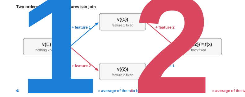
The average extra contribution of $i$ over all orders in which the features can join.

What do the SHAP values of one prediction sum to?

Answer

${\sum }_i{\Phi }_i=f(x)-Ef(X)$

Observational vs. interventional value function?

Answer

Observational $E[f(X)\mid X_S=x_S]$: explains the data.
Interventional $E_{X_{\bar{S}}}f(x_S,X_{\bar{S}})$: explains the model.

Interventional SHAP for a GAM $f(x)={\sum }_i{f}_i(x_i)$?

Answer

${\Phi }_i=f_i(x_i)-E{f}_i(X_i)$: it recovers the component functions.

What is a counterfactual explanation?

Answer

The smallest change of the input that flips the decision.
It is not necessarily actionable or robust.

How does LIME work, and what is the caveat of post-hoc explanations?

Answer

Sample around $x$ and fit a local linear surrogate.
Explanations can be manipulated, and different methods disagree. For high stakes use interpretable models.

Risk levels of the EU AI Act with one example each?

Answer

Prohibited (social scoring), high (credit scoring, hiring, medical devices), limited (chatbots), minimal (spam filters).
GPAI models: systemic risk above $10^{25}$ FLOPs.

Overview: 1. Why and what kind of explanations, 2. Issues: correlations and interactions, 3. Counterfactual explanations, 4. SHAP, 5. LIME, 6. Criticism and outlook, 7. Legal issues (AI Act, GDPR, copyright, outside the EU).

(Literature: Christoph Molnar, Interpretable Machine Learning, online, as an introductory textbook.) Slide 75

Explainability for tabular data

Why explainable machine learning?

Slides 77-78

• Black-box models with millions of parameters are hard to debug and hard to trust.
• We might want to “understand” what the model does: in science, in critical applications (medicine), in society (loans, university administration).
• AI regulation requires transparency.

Explanations of why the model predicts something might serve to: debug code; establish trust (society, medicine); balance power and control between model provider and customer; give hints for concrete actions (e.g. recourse); reveal scientific insights (truth?); comply with regulation (EU AI Act, see below).

Setup and the gold standard

Slides 79-80

Setting of this section: ML on feature-based (tabular) data, not text or images, e.g. patients described by numeric values, loan applicants. The data is high-dimensional, the task classification or regression.

Interpretable ML (the gold standard)

Use models so simple that we can understand and judge their decision mechanism:

• decision trees,
• linear models $f(x)={\sum }_i{a}_i{x}_i$,
• generalized additive models (GAMs) $f(x)={\sum }_i{f}_i(x_i)$.

But simple interpretable models might not be powerful enough for complex prediction problems.

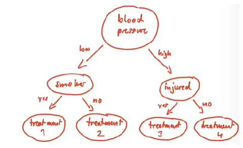
Slide 80: a decision tree is interpretable as a whole.

Local post-hoc explanations and feature attributions

Slides 81-83

Local post-hoc explanation

The model $f$ is too complex to understand as a whole. Instead we explain one particular decision with a separate explanation algorithm: it receives a point $x_0$ and the prediction $f(x_0)$, has white-box access to $f$ or can at least sample $x\in \mathcal{X}$ and query $f(x)$, and tries to justify the decision $f(x_0)$ “post hoc”. The explanation often is a feature attribution: which input features were important for this decision?

One way to build such explanations: if small changes in feature $i$ of $x$ change the decision about $x$, feature $i$ is important. Mathematically this is the gradient $\nabla f(x)$, selecting the features with the largest absolute values: gradient-based explanations.

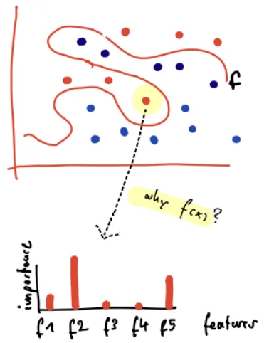
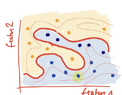
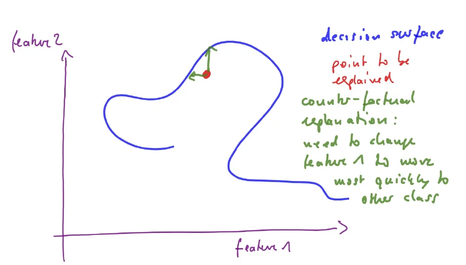
Slide 82: a feature attribution for one decision, as a bar per feature.

Slide 83: moving the yellow point along feature 1 keeps its class, along feature 2 it changes: feature 2 is more important.

Kinds of explanations

Slides 84-88

	vs.
global: understand the decision mechanism as a whole		local: explain only decisions for individual points
explain the decision function $f$ (e.g. credit decisions), the data does not matter		explain the data-generating process: relate data and decisions, e.g. find a causal reason for a disease (science)
model-specific: depends on the architecture, e.g. of a neural network		model-agnostic: SHAP, LIME, Anchors, …; no strong assumptions on $f$
data attribution: which training points were important for $f(x)$?		feature attribution: which features of $x$ were important for $f(x)$?
cooperative: provider and recipient share a goal (debugging, scientific discovery)		adversarial: different goals, e.g. a loan application; the bank has no incentive to give “true” explanations if the customer may use them to sue

Engineering vs. science of explainable AI

Slides 89-92

One can engineer many heuristics that produce explanations, and many of them “make sense”. But what scientific guarantees can we give? When is an explanation “true”? By which standard should we evaluate explanations? Which guarantees hold under which assumptions?

• The scientific approach is important for the AI Act (e.g. credit scoring), medicine and other critical applications.
• An engineering approach is justified for exploratory data analysis (science), code debugging, and whenever a useful explanation helps but even many wrong explanations do not really hurt.

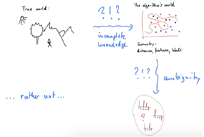
Slide 92: can we assess that an explanation is true? The algorithm only sees an incomplete picture of the world, and many different explanations fit it: rather not.

Local post-hoc explanations (feature attributions)

General issues: correlations and interactions

Slides 94-98

Before the methods, two issues that come up in many of them:

Correlated features in the data domain

Methods that isolate individual features as “reasons” get distorted if features are correlated in the input domain. Examples: the same feature twice (extreme case), years of full-time employment and gender, address and income. The model might pick one of them and ignore the others, use both with different weights, or even use both with opposite weights that cancel in the decision function but not in the gradient.

Interactions in the decision function

Features can also be coupled in the output: they interact. Examples: the XOR function (which of the two features is more important? impossible to answer, we need both), two genes that only jointly trigger a disease. More generally there are $k$-th order interactions of $k$ features. What a single importance score should do here is very unclear and may depend on tiny implementation details.

(More: Barocas, Selbst, Raghavan, “The hidden assumptions behind counterfactual explanations and principal reasons”, FAccT 2020.)

Counterfactual explanations

Slides 99-103

(Original paper: Wachter, Mittelstadt and Russell, “Counterfactual explanations without opening the black box: automated decisions and the GDPR”, 2017.)

Counterfactual explanation

What is the smallest change of the input such that the decision function returns a different result? Examples: “If your income were 500 Euro higher, you would get the credit.” “If your gender were male, you would be admitted to the program.” (?!?) One tries to find one or few features whose increase, decrease or change moves the point to the other side of the decision surface.

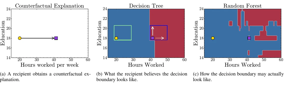
Slide 101: the counterfactual explanation says: change feature 1 to move most quickly to the other class.

Slide 102: (a) the counterfactual the recipient gets, (b) the simple, monotone boundary they imagine, (c) how a random forest's boundary may actually look. Counterfactuals of complex functions might not be robust.

Are counterfactuals helpful for recourse?

Counterfactuals are often proposed for recourse: which features to change to get accepted. But:

• “You would get the credit if you were 10 years younger.” Not actionable.
• “You would get the credit if you earned 10,000 Euros more per year.” By then you might be 5 years older, and it is unclear whether the counterfactual still holds when the age changes too. And the bank might have retrained its model in the meantime.
• For complex decision functions the recipient’s intuitive reading (monotone, stable around the counterfactual and the input) may simply be wrong (slide 102).

A counterfactual may give a hint for recourse, but not the full picture.

Task: counterfactual explanation for a linear score

Exam-style task: counterfactuals (4 P)

A bank accepts a credit application iff $s(x)=0.5\cdot \text{income}-2\cdot \text{debts}+0.1\cdot \text{age}-20\ge 0$ (income and debts in thousand Euro, age in years). Applicant: income 40, debts 3, age 30.

(a) (1 P, easy) Compute the score and the decision.

(b) (1.5 P, harder) Give the single-feature counterfactuals (change only one feature). Which one is “smallest”? Compare raw units with changes measured in standard deviations (income 15, debts 2, age 12).

(c) (1.5 P, transfer) Discuss the counterfactuals as recourse. What changes if the bank used a random forest instead of the linear score?

Solution

(a) $s=20-6+3-20=-3<0$: rejected. (1 P)

(b) Income: $+3/0.5=+6$, i.e. 46. Debts: $-3/2=-1.5$, i.e. 1.5. Age: $+3/0.1=+30$, i.e. 60. In raw units the debt change (1.5) is smallest; in standard deviations income needs $6/15=0.4$, debts $1.5/2=0.75$, age $30/12=2.5$, so income is smallest. “Smallest” depends on the chosen distance, so the explanation depends on a modeling choice. (1.5 P)

(c) Age is not actionable. Raising income takes time, and meanwhile other features (age) change: here 5 more years give $+0.5$, so only $+5$ income would be needed, but in general the effect of simultaneous changes is unclear, and the bank may retrain its model. With a random forest the boundary is fragmented and not monotone: the counterfactual point may be an isolated accepted region, nearby points (46.5 income) may be rejected again, and larger changes need not help (slide 102). (1.5 P)

SHAP

Intuition from cooperative game theory

Slides 104-106

(Original paper: Lundberg and Lee, “A unified approach to interpreting model predictions”, NeurIPS 2017; thousands of follow-up papers.)

Cooperative game theory evaluates how much influence each player has on the payoff of a coalition (Shapley values). In ML: how much does each feature contribute to the model prediction?

Vanilla idea: the payoff is the prediction $f(x)$ at a given point, the players are the features, $F$ is the set of all features. To evaluate feature $i$, consider all subsets $S\subseteq F$ of features and compare the “prediction based only on the features in $S$” with the “prediction based on $S\cup \{i\}$”: $f_{S\cup \{i\}}(x_{S\cup \{i\}})-f_S(x_S)$. Sum this over all subsets (with weights) to get the importance of feature $i$.

Definition of SHAP

Slides 107-108

SHAP value

The SHAP value of feature $i$ of $f$ at $x$ is

$${\Phi }_i(f,x)=\sum _{S\subseteq F\setminus \{i\}}\frac{|S|!(|F|-|S|-1)!}{|F|!}\left[v\right(x,S\cup \{i\})-v(x,S)]$$

with a value function $v$ (below). The weights sum to 1 over all $S$. The values add up to ${\sum }_i{\Phi }_i=v(x,F)-v(x,\varnothing )=f(x)-Ef(X)$ (efficiency).

Weights for $|F|=2$: $\frac{1}{2},\frac{1}{2}$. For $|F|=3$: $\frac{1}{3}$ for $|S|=0$, $\frac{1}{6}$ for each of the two $|S|=1$, $\frac{1}{3}$ for $|S|=2$.

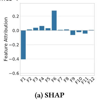
This gives importance scores for all features, plotted as a bar chart, and we “select the important ones” (at least, this is the story).

Slide 108: SHAP attributions of one decision as a bar chart.

Memory aid

SHAP = the average extra contribution of feature $i$ over all orders in which the features could join the team.

Illustration with pizza

Slides 109-111

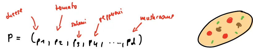
• Which toppings are most influential for the taste of a particular pizza? There are $d$ possible toppings; a pizza is a binary vector $p=(0,1,1,0,0,\dots ,1)$ saying which toppings are on it. Its taste $f(p)$ is a number between 1 and 10, say.
• For a set $S$ of toppings, $p_S$ are the values of $p$ at the coordinates $S$ (e.g. $S=\{1,3,4\}$, $p=(1,1,0,0,0,1)$ gives $p_S=(1,0,0)$).
• The value function rates the contribution of the toppings $p_S$ to the taste: look at all pizzas $P$ that agree with $p$ on $S$, $P_S=p_S$, and average their taste: $v(p,S):=E(f(P)\mid P_S=p_S)$. (Tricky detail: which average exactly? See observational vs. interventional.)
• Importance of topping $i$: compare $v(S\cup \{i\})-v(S)$ for all $S$ and sum as in the SHAP formula.

Slide 109: a pizza as a binary vector of toppings.

Observational vs. interventional SHAP

Slides 112-116

Observational value function

Fix $x$ and $S$. Average $f$ over all points whose $S$-features coincide with those of $x$:

$$v_{obs}(x,S)=E[f(X)\mid X_S=x_S]=\int f(x_S,x_{\bar{S}})p(x_{\bar{S}}\mid x_S)d{x}_{\bar{S}}$$

($\bar{S}$ the complement of $S$). Easy in theory, super difficult in practice: estimating the conditional distributions needs a huge amount of data. Pizza: for $S=\{\text{mushrooms},\text{ham}\}$ and $p_S=(1,1)$, average the taste over all pizzas on the menu with mushrooms and ham. If no pizza on the menu has mushrooms, ham and pineapple, such a pizza does not enter the average.

Interventional (marginal) value function

$$\begin{array}{rl}{v}_{int}(x,S)& =E_X[f(X)\mid do(X_S=x_S)]\\ & =E_{X_{\bar{S}}}f(x_S,X_{\bar{S}})=\int f(x_S,x_{\bar{S}})p(x_{\bar{S}})d{x}_{\bar{S}}\end{array}$$

Set $X_S$ to $x_S$ and sample the remaining features from their marginal distribution: all dependencies between $S$ and $\bar{S}$ are broken. “Interventional” because we intervene with the do-operator. Pizza: take all existing pizzas and force mushrooms and ham on them; a pizza with pineapple enters the average with mushrooms and ham added, even if such a pizza is not on the menu (out of distribution).

Which one?

Pretty much everybody uses interventional SHAP: sampling is simple. But it evaluates $f$ at out-of-distribution points and breaks dependencies, which may be questionable. If the features are independent, both value functions coincide.

Memory aid

Observational explains the data (conditions on what is known), interventional explains the model (forces values, even unrealistic combinations).

SHAP recovers GAM components

Slides 117-121

A GAM is $f(x)=c_0+{\sum }_{i=1}^d{f}_i(x_i)$ with component or shape functions $f_i$, typically non-linear (small trees, low-order polynomials).

Theorem 1 (SHAP for GAMs)

Let $f$ be a GAM with centered components, $E(f_i(X_i))=0$. Then the interventional SHAP values are the component functions:

$${\Phi }_i(f,x)=f_i(x_i).$$

Without centering, ${\Phi }_i=f_i(x_i)-E{f}_i(X_i)$. For observational SHAP the same holds if the features are independent (then both coincide).

Proof of Theorem 1

Because $f$ is a GAM,

$$v(S;x)=E_{X_{\bar{S}}}(c_0+\sum _{j\in S}{f}_j(x_j)+\sum _{j\in \bar{S}}{f}_j(X_j))=c_0+\sum _{j\in S}{f}_j(x_j)+\sum _{j\in \bar{S}}E{f}_j(X_j).$$

Taking the difference, most terms cancel: $v(S\cup \{i\};x)-v(S;x)=f_i(x_i)-E{f}_i(X_i)$, which does not depend on $S$. With the Shapley weights $w_{|S|}$:

$${\Phi }_i(x)=\sum _{S\subseteq F\setminus \{i\}}{w}_{|S|}(f_i(x_i)-E{f}_i(X_i))=(f_i(x_i)-E{f}_i(X_i))\sum _{S\subseteq F\setminus \{i\}}{w}_{|S|}=f_i(x_i)-E{f}_i(X_i),$$

since the weights sum to 1. With centered components $E{f}_i(X_i)=0$. $\square$

What it means in practice: SHAP values are meaningful if the function is a GAM and you use interventional SHAP. They might be misleading if the function is not a GAM. Similar relations hold for higher-order GAMs and higher-order SHAP values (Bordt and von Luxburg, “From Shapley values to generalized additive models and back”, AISTATS 2023).

Task: SHAP values by hand

Exam-style task: SHAP for two binary features (4 P)

Math: (conditional) expectation · SHAP weights

$x_1,x_2\in \{0,1\}$ independent with $P(X_j=1)=\frac{1}{2}$, model $f(x)=2x_1+x_2+3x_1{x}_2$, explain $x=(1,1)$ with interventional SHAP.

(a) (1 P, easy) Compute $v(\varnothing )$, $v(\{1\})$, $v(\{2\})$ and $v(\{1,2\})$.

(b) (1.5 P, harder) Compute ${\Phi }_1$ and ${\Phi }_2$ and check efficiency. How is the interaction term split?

(c) (1.5 P, transfer) New model $f(x)=x_1$, and in the data $x_2$ is an exact copy of $x_1$ ($P(X_1=1)=\frac{1}{2}$). Compute interventional and observational SHAP at $x=(1,1)$ and interpret.

Solution

(a) $v(\varnothing )=Ef=2\cdot \frac{1}{2}+\frac{1}{2}+3\cdot \frac{1}{4}=2.25$. $v(\{1\})=Ef(1,X_2)=2+\frac{1}{2}+\frac{3}{2}=4$. $v(\{2\})=Ef(X_1,1)=1+1+\frac{3}{2}=3.5$. $v(\{1,2\})=f(1,1)=6$. (1 P)

(b) Two features, weights $\frac{1}{2}$: ${\Phi }_1=\frac{1}{2}(4-2.25)+\frac{1}{2}(6-3.5)=0.875+1.25=2.125$, ${\Phi }_2=\frac{1}{2}(3.5-2.25)+\frac{1}{2}(6-4)=0.625+1=1.625$. Sum $3.75=f(x)-v(\varnothing )=6-2.25$ ✓. Main effects $2(1-\frac{1}{2})=1$ and $1\cdot (1-\frac{1}{2})=0.5$; the interaction part $3-0.75=2.25$ is split equally, $1.125$ each. The bars do not show that it is an interaction. (1.5 P)

(c) Interventional: $v(\varnothing )=0.5$, $v(\{1\})=1$, $v(\{2\})=Ef(X_1,1)=0.5$, $v(\{1,2\})=1$, so ${\Phi }_1=\frac{1}{2}(0.5)+\frac{1}{2}(0.5)=0.5$, ${\Phi }_2=0$. Observational: $v(\{2\})=E[X_1\mid X_2=1]=1$, so ${\Phi }_1=\frac{1}{2}(0.5)+\frac{1}{2}(0)=0.25$ and ${\Phi }_2=\frac{1}{2}(0.5)+\frac{1}{2}(0)=0.25$. Observational SHAP gives the unused duplicate the same importance as the used feature (it explains the data), interventional SHAP only credits $x_1$ (it explains $f$). With dependent features the two answers differ and the ranking can mislead. (1.5 P)

Practice: SHAP values by hand

Choose a model (coefficients of all terms) and a data distribution over the eight binary points, pick x, and switch between interventional and observational SHAP. The table lists every subset S with its weight and value difference, so each step of the formula can be checked.

Presets: the task example, a GAM (Theorem 1: SHAP for GAMs), XOR, an unused duplicate feature and a duplicate with opposite weights (slide 96).

SHAP with interactions and dependencies

Slides 122-127

• Interactions (California housing): longitude and latitude alone are not very informative, but jointly they tell whether a house is at the beach, which makes it much more expensive. A GAM cannot describe this; it needs an interaction term. Yet SHAP attributes a medium importance to both and ignores the interaction.
• Dependencies: a separate feature “ocean proximity” can be replaced by longitude and latitude; the variables are highly dependent. SHAP tends to distribute the importance over all dependent variables, which makes each individual value pretty meaningless.
• Rankings can be meaningless: because of both effects, truly important features can get a low rank because they are correlated with others. Picking the features with the highest SHAP scores is not a good idea for feature selection.
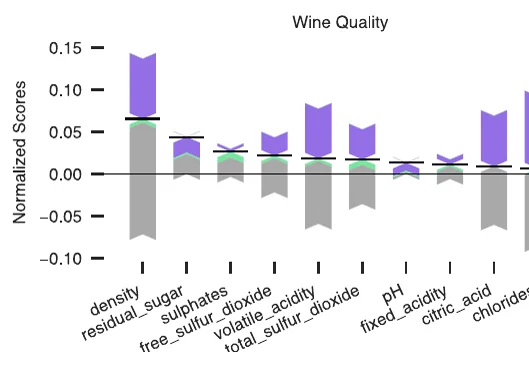
• Instead one can estimate the effects separately: standalone contribution, dependencies, interactions (DIP decomposition; König, Günther, von Luxburg, “Disentangling interactions and dependencies in feature attribution”, AISTATS 2025). Wine data: the original scores suggest density and residual sugar are most relevant and citric acid irrelevant. The decomposition shows that residual sugar matters through cooperation: sugar and density are positively correlated (sugar increases density) but have opposing effects on quality that cancel unless both are observed.

Slide 125: DIP decomposition of feature scores on the wine data: standalone contribution (gray), dependencies (purple), interactions (green).

The lecturer's conclusion: avoid SHAP whenever possible

• SHAP is very widely used because it has a nice story (game theory) and easy code with nice plots.
• SHAP is nice for GAMs, but for GAMs we might not need local interpretability methods.
• In general SHAP can be super misleading, and this is not easy to fix; the literature is full of misinterpretations.
• Unless you really know what you are doing, avoid SHAP. Many criticisms (correlations, interactions) also concern other feature attribution methods.

LIME

LIME on tabular data and images

Slides 128-133

(Ribeiro, Singh, Guestrin, “Why should I trust you? Explaining the predictions of any classifier”, SIGKDD 2016; Garreau and von Luxburg, “Explaining the explainer: a first theoretical analysis of LIME”, AISTATS 2020; Bordt, Upadhyay, Akata, von Luxburg, “The manifold hypothesis for gradient-based explanations”, 2022.)

LIME (Local Interpretable Model-agnostic Explanations)

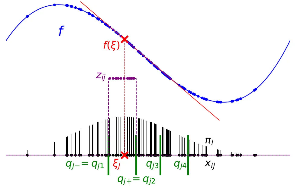
We cannot replace a complex function $f$ (random forest, deep network) globally by a simple function on few “explainable” features (it would not be accurate). But we might approximate it locally by a simple linear function to understand the decision at $x$, hoping that this local approximation is meaningful. Rough sketch for tabular data (${\mathbb{R}}^d$):

1. Fix the point $x$ whose decision should be explained.
2. Sample points $x_1,\dots ,x_m$ locally around $x$, evaluate $f(x_1),\dots ,f(x_m)$, apply a binning procedure to the features.
3. Fit a simple linear function that approximates $f$ locally.
4. Use the few most prominent coordinates of this linear model as the explanation.

LIME only needs to evaluate $f$ at arbitrary inputs: it works for any black box.

Slide 131: LIME on tabular data. Samples around the point (weights as vertical bars) are binned (green boundaries), and a linear model (red) approximates f locally.

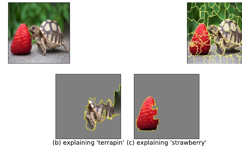
Images: pixels are not interpretable features. The image is split into superpixels (contiguous patches, e.g. $d=64$) in a pre-processing step. LIME samples images near the given one by randomly switching superpixels on and off; the binary on/off vector plays the role of the feature vector. It then identifies the superpixels that contribute most to the classification.

Slide 132: LIME on an image. Superpixels explaining "terrapin" and "strawberry".

Criticism and outlook

Explanations can be manipulated

Slides 134-137

(Anders et al., “Fairwashing explanations with off-manifold detergent”, ICML 2020; Slack et al., “Fooling LIME and SHAP: adversarial attacks on post hoc explanation methods”, AIES 2020; Slack et al., “Counterfactual explanations can be manipulated”, 2021. More general: Rudin, “Stop explaining black box machine learning models for high stakes decisions and use interpretable models instead”, Nature Machine Intelligence 2019; Bordt, Finck, Raidl, von Luxburg, “Post-hoc explanations fail to achieve their purpose in adversarial contexts”, FAccT 2022.)

How manipulation works

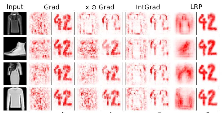
Given $f$, construct $\tilde{f}$ that makes the same decisions on the data but behaves very differently off the data distribution. Real data often lives on a low-dimensional manifold; around each data point there are many off-manifold points. Explanation algorithms sample from a neighborhood of $x_0$, often off-manifold (or use gradients). By changing $\tilde{f}$ off-manifold we change the explanation at $x_0$ without changing any decision.

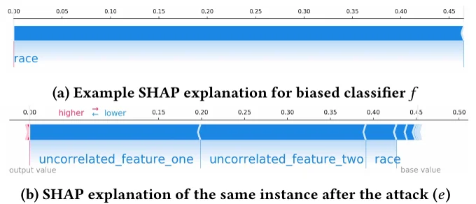
Slide 136: manipulated gradient-based explanations always show "42" (Anders et al.).

Slide 137: a classifier that heavily uses "race" gets an innocent-looking SHAP explanation after the attack (Slack et al.).

Different algorithms, different explanations

Slides 138-141

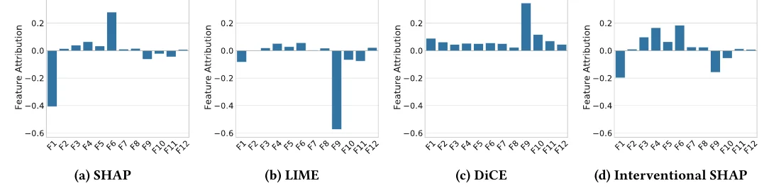
Slide 138: SHAP, LIME, DiCE and interventional SHAP explain the same decision of the same model completely differently (Bordt et al., FAccT 2022).

• In an adversarial setting the “opponent” can cherry-pick the explanation they like; for an examiner this is pretty much impossible to detect. We cannot trust these explanations if we don’t trust the one who invokes the algorithm.
• Informative explanations only exist for simple functions: in a framework for when a local explanation is “informative”, one can prove this, questioning the whole point of local post-hoc explanations (Günther, Szabados, Bhattacharjee, Bordt, von Luxburg, arXiv 2025).
• Explanation cards (Günther, Szabados, König, Meding, Bordt, von Luxburg, arXiv 2026), the constructive way forward: augment explanations with information about robustness and validity and clear instructions for interpretation. This can make otherwise uninformative explanations useful, helps detect when they are not, and shifts responsibility from users to providers, who must state upfront what can and cannot be concluded.

The lecturer's summary

If explanations are designed for a different end user, supply explanation cards. If reliable explanations matter (e.g. in a societal context), use interpretable algorithms, do not allow complicated models with post-hoc explanations. Other people have different opinions here.

Outlook: images, language models, mechanistic interpretability

Slides 142-144

• Image classifiers: many methods, many based on the gradient of the output with respect to the input pixels (which pixels affect the prediction most): saliency maps (Simonyan et al., ICLR Workshop 2014), integrated gradients (Sundararajan et al., ICML 2017), Grad-CAM (Selvaraju et al., ICCV 2017), SmoothGrad (Smilkov et al., 2017).
• Language models: people ask LLMs to explain themselves or their reasoning. The lecturer is not convinced, and it is definitely not trustworthy when the explanation really matters. A vastly open field.
• Mechanistic interpretability: try to extract what sub-components of a trained network do, e.g. which sub-task a particular attention head performs. Some small successes, but big questions: does it generalize beyond toy applications, and how trustworthy are the findings?

Legal issues

Why regulate, and how legislation works

Slides 147-148

Reasons for regulating AI systems:

• Safety and harm prevention: AI can cause accidents, discrimination etc. at scale.
• Accountability: who is liable when an AI system causes harm?
• Fundamental rights: privacy, non-discrimination.
• Market integrity: consumer protection, a level playing field.
• Trust: public acceptance of AI requires oversight and legal certainty.

How legislation works: law sets norms and principles at a high level, not technical specifications. It does not define how to comply; that is left to standards bodies, industry guidelines and case law. Many key concepts are deliberately vague (what does “transparent” mean for an ML model?), and their interpretation is refined over time by court rulings and national regulators. Compliance is an ongoing process, not a one-time checklist.

The EU AI Act

Slides 150-155

• The world’s first comprehensive AI regulation. It applies to providers, deployers and importers of AI systems placed on the EU market or affecting persons in the EU.
• Goals: AI that is safe, transparent and non-discriminatory; innovation through legal certainty.
• Timeline: proposed April 2021, political agreement December 2023, in force August 2024, stepwise roll-out until August 2026.
• Reading it: the full text starts with the non-binding recitals (background, motivation, aims, interpretation); the legally binding part starts in the middle (“Chapter I: General provisions”).

Risk-based approach

The AI Act does not regulate “algorithms” but their applications, sorted into risk categories:

• Unacceptable risk (prohibited): real-time biometric surveillance in public spaces, social scoring by governments, subliminal manipulation, exploitation of vulnerable groups.
• High risk: safety-critical systems (medical devices, critical infrastructure, autonomous vehicles) and high-impact systems (credit scoring, recruitment, education, law enforcement, border control).
• Limited risk (chatbots, deepfakes) and minimal risk (recommender systems, spam filters, games): little or no mandatory obligations.

The major part of the AI Act is about high-risk systems.

Obligations for high-risk systems

Risk management over the entire lifecycle; data governance (high-quality training, validation and test data, documented data practices); technical documentation and automatic logging; transparency toward deployers and instructions for use; human oversight (humans can intervene or override).

General-purpose AI (GPAI) models

Added only in the last round of debates, because ChatGPT entered the market. Article 3(63): “an AI model that is trained with a large amount of data using self-supervision at scale, that displays significant generality and is capable of competently performing a wide range of distinct tasks regardless of the way the model is placed on the market and that can be integrated into a variety of downstream systems or applications, except AI models that are used for research, development or prototyping activities before they are placed on the market.”

• Systemic risk threshold: training compute $>10^{25}$ FLOPs (roughly GPT-4 scale and above).
• All GPAI providers: technical documentation, comply with copyright law, publish a summary of the training data.
• Systemic-risk models additionally: adversarial testing / red-teaming before release, reporting serious incidents to the European Commission, cybersecurity measures, energy efficiency reporting.

Practice: which risk category?

Fourteen applications written for these notes. Pick the risk category as the lecture defines it; the explanation points to the slide. The legal text has exceptions and details beyond the lecture.

GDPR

Slides 157-159

• The General Data Protection Regulation: EU regulation in force since May 2018, regulating the processing of personal data of natural persons. It applies to any entity processing personal data of EU residents, wherever the entity is located. Relevance for ML: training data frequently contains personal data.
• Data consent: lawful reasons for processing are consent, contract, legal obligation, legitimate interest, … Special categories (health, biometrics, ethnicity, political opinions, …) need explicit consent. Data minimization: collect only what is necessary for the stated purpose. Purpose limitation: data may not be reused beyond the original purpose. ML implication: scraping publicly available data does not automatically grant permission to use it for training.
• Right to be forgotten: individuals can request the erasure of their personal data. Once data is encoded in model weights, deletion is non-trivial; active research area machine unlearning: removing the influence of specific training points from a model.

Intellectual property and copyright

Slides 161-162

• Training data (EU Copyright Directive 2019): using any data needs a legal basis: a license, public domain or open licenses (Creative Commons), own data, a data sharing agreement, … GDPR applies additionally for personal data. Scraping without permission is increasingly contested, e.g. New York Times v. OpenAI, Getty Images v. Stability AI.
• Ownership of AI output: current consensus: no copyright without human authorship; AI has no legal personhood.
• Training as copyright infringement: an active legal dispute, not yet settled by courts in the US or the EU.
• Trade secrets: model weights and training pipelines can be protected as proprietary IP.
• Patents: an AI cannot be listed as inventor.

Regulation outside the EU and take-aways

Slides 164-165

• UK: no dedicated AI law; existing sector regulators cover many cases.
• Canada: relies on existing privacy, consumer protection, human rights and sector rules (an attempt at AI regulation was stopped in 2025).
• USA: no federal AI law; sector-specific rules (medical AI, consumer protection, discrimination, …).
• China: Algorithmic Recommendation Provisions (2022), Generative AI Regulation (2023); emphasis on content control and alignment with state interests.
• No global consensus on regulation.

Key take-aways

• Know your data: legal basis, provenance, personal data.
• Know your system: its risk category under the AI Act and the resulting obligations.
• Know your outputs: generated content carries copyright risk for the deployer.

The legal landscape is evolving rapidly; landmark court decisions and implementing regulations are still pending.

Summary

Topic	Key message
why explain	debugging, trust, power balance, recourse, science, regulation; gold standard: interpretable models (trees, linear, GAMs)
local post-hoc	an extra algorithm explains one decision $f(x_0)$, usually as feature attributions (e.g. gradients)
kinds	global/local, function/data, model-specific/agnostic, data/feature attribution, cooperative/adversarial
issues	correlated features and interactions make importance ill-defined
counterfactuals	smallest change that flips the decision; depends on the metric, not always actionable or robust
SHAP	Shapley-weighted average of $v(S\cup \{i\})-v(S)$; observational $E[f\mid X_S=x_S]$ vs. interventional $Ef(x_S,X_{\bar{S}})$; recovers GAM components; misleading with interactions and dependencies
LIME	local linear surrogate from samples around $x$ (bins, superpixels)
criticism	manipulation off-manifold, algorithms disagree, cherry-picking, informative only for simple functions; explanation cards
AI Act	applications by risk: prohibited, high (obligations), limited, minimal; GPAI, systemic risk $>10^{25}$ FLOPs
GDPR, copyright	lawful basis and consent, minimization, purpose limitation, right to be forgotten (unlearning); training data needs a legal basis, no copyright without a human author

Self-Test

Question cards (12)

What is the difference between an interpretable model and a local post-hoc explanation?

Answer

An interpretable model (tree, linear model, GAM) is simple enough to understand its whole decision mechanism. A local post-hoc explanation uses a separate algorithm to justify one decision $f(x_0)$ of a model that is too complex to understand.

Why do correlated features and interactions cause problems for feature importance scores?

Answer

Correlated features can substitute each other, so the model may use either, both, or both with cancelling weights, and scores distribute or misplace importance. With interactions (XOR, two genes) no single feature is important alone, so a per-feature score is ill-defined.

What is a counterfactual explanation, and why is it limited as recourse?

Answer

The smallest input change that flips the decision. It may be non-actionable (age), other features change meanwhile, the model may be retrained, “smallest” depends on the metric, and for complex models the counterfactual need not be stable or monotone.

Write down the SHAP formula and explain the weights.

Answer

${\Phi }_i={\sum }_{S\subseteq F\setminus \{i\}}\frac{|S|!(|F|-|S|-1)!}{|F|!}[v(S\cup \{i\})-v(S)]$. The weight is the fraction of feature orderings in which exactly the features of $S$ come before $i$; the weights sum to 1.

Define the observational and the interventional value function. When do they coincide?

Answer

$v_{obs}(x,S)=E[f(X)\mid X_S=x_S]$ (conditional distribution of the rest), $v_{int}(x,S)=E_{X_{\bar{S}}}f(x_S,X_{\bar{S}})$ (marginal of the rest, breaks dependencies, out-of-distribution points). They coincide if the features are independent.

State Theorem 1 (SHAP for GAMs) and the key step of the proof.

Answer

For a GAM with centered components, interventional SHAP gives ${\Phi }_i=f_i(x_i)$. Key step: $v(S\cup \{i\})-v(S)=f_i(x_i)-E{f}_i(X_i)$ does not depend on $S$, and the weights sum to 1.

What does SHAP report for the house price example with longitude and latitude, and why is it misleading?

Answer

A medium importance for both, while the real effect is their interaction (being at the beach). With a dependent third feature (ocean proximity) importance is spread further. The ranking says little about what matters.

How does LIME work on tabular data and on images?

Answer

Sample points around $x$, evaluate $f$, bin the features and fit a local linear model; its largest coefficients are the explanation. For images the features are superpixels switched on and off.

How can an explanation be manipulated without changing the model's decisions?

Answer

Keep $f$ on the data manifold but change it off-manifold. Explanation methods sample (or take gradients) in neighborhoods that leave the manifold, so the explanation changes while all decisions on real data stay the same.

What are explanation cards?

Answer

Explanations augmented with information about robustness and validity and with interpretation instructions, so providers state upfront what can be concluded; this shifts responsibility from users to providers.

Name the risk categories of the EU AI Act with an example each, and the obligations for high-risk systems.

Answer

Prohibited (social scoring by governments), high (credit scoring, recruitment, medical devices), limited (chatbots, deepfakes), minimal (spam filters, games). High risk: risk management, data governance, documentation and logging, transparency, human oversight.

Which GDPR principles matter for ML training data?

Answer

A lawful basis (consent etc., explicit consent for special categories), data minimization, purpose limitation, and the right to be forgotten, which is hard once data is in the weights (machine unlearning). Public availability does not imply permission to train on the data.

Multiple Choice

Multiple choice (8)

Two binary features, independent and uniform; $f(x)=4x_1$. What is the interventional SHAP value ${\Phi }_1$ at $x=(1,0)$?

• 4

• 2

• 1

• 0

Explanation

GAM: ${\Phi }_1=f_1(x_1)-E{f}_1(X_1)=4-2=2$ (Theorem 1: SHAP for GAMs without centering). ${\Phi }_2=0$.

Which statement about interventional SHAP is true?

• It conditions on $X_S=x_S$ and averages over the conditional distribution.

• It samples the remaining features from their marginal distribution and can evaluate $f$ at out-of-distribution points.

• It needs a causal model of the data.

• It always equals observational SHAP.

Explanation

$v_{int}(x,S)=E_{X_{\bar{S}}}f(x_S,X_{\bar{S}})$. It coincides with observational SHAP only for independent features.

In the data, $x_2$ is an exact copy of $x_1$, and the model is $f(x)=x_1$. Observational SHAP gives

• all importance to $x_1$

• all importance to $x_2$

• equal importance to $x_1$ and $x_2$

• zero importance to both

Explanation

Conditioning on $x_2$ reveals $x_1$, so both get the same credit; interventional SHAP would give $x_2$ zero.

What does LIME fit to explain a decision at $x$?

• a global decision tree on all training data

• a simple linear model on samples drawn around $x$

• the Shapley values of all feature subsets

• the gradient of the loss with respect to the training points

Explanation

Local Interpretable Model-agnostic Explanations: local linear surrogate on binned features or superpixels.

Why can explanations be manipulated without changing any decision on the data?

• Because SHAP is randomized.

• Because explanation methods query the model off the data manifold, where it can be changed freely.

• Because the model can be retrained with different labels.

• Because counterfactuals are always unique.

Explanation

Anders et al. 2020, Slack et al. 2020: keep $f$ on the manifold, change it off-manifold.

Under the EU AI Act as presented, a credit scoring system is

• prohibited

• high risk

• limited risk

• minimal risk

Explanation

Credit scoring is a high-impact system (slide 152) with obligations for risk management, data governance, documentation, transparency and human oversight.

A general-purpose model is presumed to have systemic risk under the AI Act if its training compute exceeds about

• $10^{15}$ FLOPs

• $10^{20}$ FLOPs

• $10^{25}$ FLOPs

• $10^{30}$ FLOPs

Explanation

Slide 154: roughly GPT-4 scale and above.

Which statement about data and copyright is correct according to the lecture?

• Publicly available data may always be used for training.

• AI-generated output is copyrighted by the model provider.

• Using data for training needs a legal basis, and GDPR applies additionally to personal data.

• An AI system can be listed as inventor on a patent.

Explanation

Scraping does not automatically grant permission; no copyright without human authorship; AI cannot be an inventor.

Cheat sheet and full integration tasks

The first task covers the two calculations of this lecture, SHAP values and a counterfactual for a linear score. The second is one scenario in which the terms on explanation methods, the AI Act and the GDPR have to be applied once. Write your own sheet first, solve the tasks with it next to you, then open the sheet at the bottom and compare. The letters in brackets name the block of the sheet that a subtask needs.

Full integration task: SHAP and a counterfactual by hand (14 P)

Math: (conditional) expectation · SHAP weights

Part 1. $x_1,x_2\in \{0,1\}$ independent with $P(X_j=1)=\frac{1}{2}$. The model is $f(x)=x_1+3x_2+2x_1{x}_2$. Explain the point $x=(1,0)$ with interventional SHAP.

(a) (3 P, block A) Compute $v(\varnothing )$, $v(\{1\})$, $v(\{2\})$ and $v(\{1,2\})$.

(b) (3 P, block A) Compute ${\Phi }_1$ and ${\Phi }_2$ and check efficiency. What does the sign of ${\Phi }_2$ say?

(c) (2 P, block A) Drop the interaction term, $g(x)=x_1+3x_2$. Give the SHAP values of $g$ at $(1,0)$ without a calculation over subsets. Which part of ${\Phi }_1$ and ${\Phi }_2$ in (b) comes from the interaction?

Part 2. A bank accepts a credit application iff $s(x)=0.4\cdot \text{income}-1.5\cdot \text{debts}+0.2\cdot \text{years employed}-18\ge 0$ (income and debts in thousand Euro). Applicant: income 35, debts 4, 10 years employed.

(d) (3 P, block B) Compute the score and the decision. Give the counterfactual for each single feature, if one exists.

(e) (3 P, block B) Which single-feature counterfactual is smallest when changes are measured in standard deviations (income 10, years employed 8)? Give a counterfactual that changes two features and uses the debts. Discuss both as recourse.

Solution

(a) Fix the features in $S$ at the values of $x$ and average over the others. $v(\varnothing )=Ef=\frac{1}{2}+\frac{3}{2}+2\cdot \frac{1}{4}=2.5$. $v(\{1\})=Ef(1,X_2)=1+\frac{3}{2}+1=3.5$. $v(\{2\})=Ef(X_1,0)=\frac{1}{2}$. $v(\{1,2\})=f(1,0)=1$. (3 P)

(b) ${\Phi }_1=\frac{1}{2}(3.5-2.5)+\frac{1}{2}(1-0.5)=0.5+0.25=0.75$. ${\Phi }_2=\frac{1}{2}(0.5-2.5)+\frac{1}{2}(1-3.5)=-1-1.25=-2.25$. Sum $-1.5=f(x)-v(\varnothing )=1-2.5$. ${\Phi }_2$ is negative: $x_2=0$ pulls the prediction below the average prediction. (3 P)

(c) $g$ is a GAM, so ${\Phi }_i=g_i(x_i)-E{g}_i(X_i)$: ${\Phi }_1=1-0.5=0.5$ and ${\Phi }_2=0-1.5=-1.5$. The rest comes from the interaction: $0.75-0.5=0.25$ for feature 1 and $-2.25+1.5=-0.75$ for feature 2, together $-0.5$, which is $2x_1{x}_2-E(2X_1{X}_2)=0-0.5$. The two bars do not show that an interaction is involved. (2 P)

(d) $s=14-6+2-18=-8<0$: rejected. The score has to rise by 8. Income: $+8/0.4=+20$, that is 55. Years employed: $+8/0.2=+40$, that is 50 years. Debts: $-8/1.5\approx -5.3$, but the debts are only 4, and paying them off completely gains just 6. There is no counterfactual in the debts alone. (3 P)

(e) Income: $20/10=2$ standard deviations. Years employed: $40/8=5$. Income is the smallest single change. Two features: pay off all debts ($+6$) and raise the income by $2/0.4=5$ to 40. As recourse: 40 more years of employment is not actionable. A higher income takes time, during which the years employed grow as well and the bank may retrain its model. The combined change is the most realistic one, but which counterfactual counts as “smallest” depends on the chosen distance. (3 P)

Full integration task: one credit model, every term (10 P)

A bank uses a random forest for credit decisions. Rejected applicants receive a bar chart of SHAP values as the explanation.

(a) (2 P, block C) Classify this explanation: global or local, model-specific or model-agnostic, data or feature attribution, cooperative or adversarial setting?

(b) (2 P, blocks A and C) The features “address” and “income” are strongly correlated. What does that do to the SHAP values, and where do observational and interventional SHAP differ?

(c) (2 P, block C) How could the bank change the explanations without changing a single decision? What does the lecture recommend where reliable explanations matter?

(d) (2 P, block D) Which risk category of the EU AI Act does credit scoring fall into, and which obligations follow? Give the category of a customer service chatbot, of social scoring by a government and of a spam filter.

(e) (2 P, block E) An applicant asks the bank to delete their personal data, which was used to train the model. And the bank had collected public social media profiles as extra training data. What does the GDPR say to both?

Solution

(a) Local (one decision), post-hoc and model-agnostic (SHAP only needs to evaluate $f$), a feature attribution. The setting is adversarial: the bank and the rejected applicant have different goals. (2 P)

(b) SHAP spreads the importance over the dependent features, so each single value means little and the ranking can mislead. Observational SHAP conditions on the known features and gives credit to a correlated feature even if the model does not use it: it explains the data. Interventional SHAP breaks the dependence, evaluates $f$ at unrealistic combinations and only credits what the model uses: it explains the model. With independent features both agree. (2 P)

(c) Build a model that makes the same decisions on the data but behaves differently off the data manifold. Explanation methods sample around the point, mostly off the manifold, so the explanation changes while the decisions stay. The bank can also pick the explanation method it likes. Recommendation: use interpretable models (trees, linear models, GAMs) where explanations matter, or supply explanation cards that state what can be concluded. (2 P)

(d) Credit scoring is high risk. Obligations: risk management over the lifecycle, data governance, technical documentation and logging, transparency towards deployers, human oversight. Chatbot: limited risk. Social scoring by a government: unacceptable risk, prohibited. Spam filter: minimal risk. (2 P)

(e) The applicant has the right to erasure (right to be forgotten). Data that is encoded in model weights is hard to remove, which is the topic of machine unlearning. Public availability does not grant permission to use data for training: the bank needs a lawful basis, must respect purpose limitation and data minimization, and needs explicit consent for special categories such as health or ethnicity. (2 P)

Cheat sheet: explainability and law (6 blocks)

A. SHAP by hand for two features

1. Value function (interventional): $v(S)=Ef(x_S,X_{\bar{S}})$. Fix the features in $S$ at the values of the explained point and average over the others.
2. Four values: $v(\varnothing )=Ef(X)$, $v(\{1\})$, $v(\{2\})$ and $v(\{1,2\})=f(x)$.
3. ${\Phi }_1=\frac{1}{2}[v(\{1\})-v(\varnothing )]+\frac{1}{2}[v(\{1,2\})-v(\{2\})]$ and ${\Phi }_2=\frac{1}{2}[v(\{2\})-v(\varnothing )]+\frac{1}{2}[v(\{1,2\})-v(\{1\})]$.
4. Check (efficiency): ${\Phi }_1+{\Phi }_2=f(x)-v(\varnothing )$.

SHAP for two features: the average gain of a feature over the two orders in which the features can be added.

You see	It means
independent binary features with $P(X_j=1)=p_j$	$E(X_j)=p_j$ and $E(X_1{X}_2)=p_1{p}_2$
a model without interaction terms (a GAM)	${\Phi }_i=f_i(x_i)-E{f}_i(X_i)$, no subsets needed
an interaction term	its contribution is shared between the features, and the bars do not show it
a negative SHAP value	this feature value pulls the prediction below the average prediction
dependent features	observational and interventional SHAP differ: observational credits an unused copy, interventional does not
three features	weights $\frac{1}{3}$ for $|S|=0$, $\frac{1}{6}$ for each $|S|=1$, $\frac{1}{3}$ for $|S|=2$

B. Counterfactual for a linear score

• Score $s(x)={\sum }_i{a}_i{x}_i+c$, accepted iff $s(x)\ge 0$. A rejected point has to gain $-s(x)$.
• One feature alone: ${\Delta }_i=\frac{-s(x)}{a_i}$. Check that the new value is possible (debts cannot go below 0).
• Smallest change: compare $|{\Delta }_i|$ in raw units or $|{\Delta }_i|/{\sigma }_i$ in standard deviations. The answer depends on this choice.
• Several features: the gains add up, ${\sum }_i{a}_i{\Delta }_i=-s(x)$.
• Recourse checks: is the change actionable, does it still hold after the time it takes, has the model changed in the meantime, is the decision function monotone around the point?

C. Methods and their problems

You see	It means
a tree, a linear model or a GAM	interpretable model, the gold standard
an extra algorithm explains one decision $f(x_0)$	local post-hoc explanation, usually a feature attribution
only evaluations of $f$ are needed	model-agnostic: SHAP, LIME, counterfactuals
samples around $x$ and a local linear fit	LIME (with bins for tabular data, superpixels for images)
the smallest change that flips the decision	counterfactual explanation
correlated features	attributions are spread over them, rankings can mislead
XOR or two genes that only act together	interaction: a single importance score per feature is not defined
same decisions on the data, different function off the data	manipulated explanations
provider and recipient with different goals	adversarial setting: the provider can cherry-pick the explanation

D. EU AI Act

Risk category	Examples	Consequence
unacceptable	social scoring by governments, real-time biometric surveillance in public, subliminal manipulation	prohibited
high	credit scoring, recruitment, education, law enforcement, medical devices, critical infrastructure	risk management, data governance, documentation and logging, transparency, human oversight
limited	chatbots, deepfakes	little or no mandatory obligations
minimal	spam filters, recommender systems, games	little or no mandatory obligations

• The Act regulates applications, not algorithms.
• General-purpose AI models: documentation, copyright compliance and a summary of the training data. Systemic risk above $10^{25}$ FLOPs of training compute: also red-teaming, incident reporting, cybersecurity.

E. GDPR and copyright

You see	It means
personal data of EU residents	the GDPR applies, wherever the processor sits
health, biometrics, ethnicity, political opinions	special categories: explicit consent
data collected “just in case” or reused for a new purpose	violates data minimization or purpose limitation
a request to delete personal data	right to be forgotten. For trained models: machine unlearning
publicly available data	not automatically allowed for training
output generated by an AI	no copyright without human authorship

F. Traps

• $v(\varnothing )$ is the average prediction $Ef(X)$, not $f(0)$.
• In $v(\{2\})$ the second feature is fixed at the value of the explained point, also if that value is 0.
• The two SHAP values must add up to $f(x)-v(\varnothing )$. If not, a value function is wrong.
• A counterfactual is not a recipe: the smallest change depends on the distance and may not be actionable.
• Credit scoring is high risk, not prohibited. Prohibited is social scoring by governments.

References

All sources cited on the slides, in slide order (26 entries)

Slide	Source	Key point
75	Molnar, Interpretable Machine Learning (online book)	textbook
98	Barocas, Selbst and Raghavan, “The hidden assumptions behind counterfactual explanations and principal reasons”, FAccT 2020	issues of attributions
99	Wachter, Mittelstadt and Russell, “Counterfactual explanations without opening the black box: automated decisions and the GDPR”, 2017	counterfactuals
104	Lundberg and Lee, “A unified approach to interpreting model predictions”, NeurIPS 2017	SHAP
121	Bordt and von Luxburg, “From Shapley values to generalized additive models and back”, AISTATS 2023	SHAP and GAMs
126	König, Günther and von Luxburg, “Disentangling interactions and dependencies in feature attribution”, AISTATS 2025	DIP decomposition
128	Ribeiro, Singh and Guestrin, “Why should I trust you? Explaining the predictions of any classifier”, SIGKDD 2016	LIME
128	Garreau and von Luxburg, “Explaining the explainer: a first theoretical analysis of LIME”, AISTATS 2020	LIME theory
128	Bordt, Upadhyay, Akata and von Luxburg, “The manifold hypothesis for gradient-based explanations”, 2022	gradients
132	Ren and Malik, 2003	superpixels
134, 136	Anders et al., “Fairwashing explanations with off-manifold detergent”, ICML 2020	manipulated gradients
134, 137	Slack et al., “Fooling LIME and SHAP: adversarial attacks on post hoc explanation methods”, AIES 2020	manipulated SHAP
134	Slack et al., “Counterfactual explanations can be manipulated”, 2021	manipulated counterfactuals
134	Rudin, “Stop explaining black box machine learning models for high stakes decisions and use interpretable models instead”, Nature Machine Intelligence 2019	interpretable models
134, 138	Bordt, Finck, Raidl and von Luxburg, “Post-hoc explanations fail to achieve their purpose in adversarial contexts”, FAccT 2022	adversarial contexts
139	Günther, Szabados, Bhattacharjee, Bordt and von Luxburg, “Informative post-hoc explanations only exist for simple functions”, arXiv 2025	impossibility
140	Günther, Szabados, König, Meding, Bordt and von Luxburg, “We need explanation cards to connect explanation algorithms to the real world”, arXiv 2026	explanation cards
142	Simonyan et al., “Deep inside convolutional networks: visualising image classification models and saliency maps”, ICLR Workshop 2014	saliency maps
142	Sundararajan et al., “Axiomatic attribution for deep networks”, ICML 2017	integrated gradients
142	Selvaraju et al., “Grad-CAM: visual explanations from deep networks via gradient-based localization”, ICCV 2017	Grad-CAM
142	Smilkov et al., “SmoothGrad: removing noise by adding noise”, arXiv 2017	SmoothGrad
151	Regulation (EU) 2024/1689, the AI Act, on EUR-Lex	full text
157	General Data Protection Regulation (GDPR), in force since May 2018	personal data
161	EU Copyright Directive, 2019	training data
161	New York Times v. OpenAI; Getty Images v. Stability AI (lawsuits)	scraping contested
164	China: Algorithmic Recommendation Provisions (2022), Generative AI Regulation (2023)	regulation outside the EU

Related

• Previous: Lecture 9.1: Fairness · Course: Overview · Formula Sheet · Glossary
• Concepts: Feature Attribution, SHAP, LIME, Counterfactual Explanation, AI Regulation, Fairness Criteria
• Exercises: Sheet 11, Exercise 1 (counterfactual explanations and algorithmic recourse), Exercise 3 (SHAP explanations and what they do not mean)