Lecture 9.1: Fairness

TL;DR

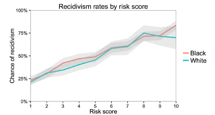
1. There is no unique definition of fairness. COMPAS is “fair” in one sense (same reoffending rate per risk score) and “unfair” in another (non-reoffending black defendants get high scores twice as often). With different base rates, no non-trivial classifier can satisfy both.
2. Sources of unfairness: minorities drown in accuracy-maximizing systems, sampling bias, pre-existing biases in the data, the choice of features, the choice of the target variable (proxy).
3. Group criteria (binary $A$, $Y$, $\hat{Y}$): demographic parity $\hat{Y}\perp A$, i.e. $P(\hat{Y}=1\mid A=0)=P(\hat{Y}=1\mid A=1)$; equalized odds $\hat{Y}\perp A\mid Y$, i.e. equal TPR and FPR (equal TPR alone = equal opportunity); predictive parity $Y\perp A\mid \hat{Y}$, i.e. equal $P(Y=1\mid \hat{Y}=y,A)$; calibration $P(Y=1\mid \hat{Y}=y,A=a)=y$.
4. Impossibility: if $A$ and $Y$ are dependent (different base rates), demographic parity and predictive parity cannot both hold, and neither can equalized odds and predictive parity.
5. Fixing unfairness: removing the sensitive attribute does not work (proxies like the ZIP code). Train with a fairness constraint (relaxations are often too loose). Post-processing: a derived classifier $P(\tilde{Y}=1\mid \hat{Y}=y,A=a)$, often randomized, or group-specific thresholds where the ROC curves intersect.
6. Tradeoffs: fairness costs accuracy, randomized decisions are questionable, feedback loops make predictions self-fulfilling. Society has to decide, technical solutions cannot settle it.

Exam relevance

• Real exam, task 3: fairness from two per-group count tables: demographic parity, TPR and FPR, equal opportunity and equalized odds, then randomized post-processing to reach equal opportunity. Known mistake: computing the TPR as $P(\hat{Y}=1\mid \dots )$ conditioned on $\hat{Y}$ instead of $Y$. Practice with the table task and the widget (random practice tables).
• Mock exam: ROC curves and equalized odds, see the ROC task.
• Know the three criteria with their conditional independence form, which ones the constant and the perfect classifier satisfy, and the impossibility propositions with their one-line proof idea.
• Sheet 11, Exercise 2 (removing a feature is not enough).
• Everything in one go: the cheat sheet with two full integration tasks at the end of this note.

Exam essentials (8 cards)

Only what you should know by heart in the exam. Click a card for the answer, or press a to go through them as flashcards. For Anki: deck of this lecture.

Demographic parity, and how to read it off a table?

Answer

$P(\hat{Y}=1\mid A=0)=P(\hat{Y}=1\mid A=1)$, i.e. $\hat{Y}\perp A$.
Per group: $(\mathrm{TP}+\mathrm{FP})/n$.

Equalized odds and equal opportunity?

Answer

Equalized odds: equal TPR and FPR in both groups ($\hat{Y}\perp A\mid Y$). Equal opportunity: equal TPR only.
$\mathrm{TPR}=\mathrm{TP}/(\mathrm{TP}+\mathrm{FN})$, $\mathrm{FPR}=\mathrm{FP}/(\mathrm{FP}+\mathrm{TN})$.

Predictive parity?

Answer

Equal $P(Y=1\mid \hat{Y},A)$ in both groups ($Y\perp A\mid \hat{Y}$).
$\mathrm{PPV}=\mathrm{TP}/(\mathrm{TP}+\mathrm{FP})$.

Which variable does each fairness criterion condition on?

Answer

Demographic parity: nothing. Equalized odds: the true label $Y$.
Predictive parity: the prediction $\hat{Y}$.

Impossibility result for fairness criteria?

Answer

If the base rates differ ($A$ and $Y$ dependent): demographic parity and predictive parity cannot both hold,
and neither can equalized odds and predictive parity.

Which criteria do a constant and a perfect classifier satisfy?

Answer

Constant $\hat{Y}$: demographic parity and equalized odds.
Perfect classifier: equalized odds and predictive parity.

Randomized post-processing: new rates and reachable points?

Answer

Per group, with $p_y=P(\tilde{Y}=1\mid \hat{Y}=y)$: ${\mathrm{TPR}}^{\prime }=p_1\mathrm{TPR}+p_0(1-\mathrm{TPR})$, same for FPR.
Reachable per group: the quadrilateral $(0,0)$, $(1,1)$, $(\mathrm{FPR},\mathrm{TPR})$, $(1-\mathrm{FPR},1-\mathrm{TPR})$.

Why does removing the sensitive attribute not make a model fair?

Answer

Other features act as proxies for it, for example the ZIP code.

Overview: 1. The discussion about fairness (COMPAS, admissions, credit, deliveries, Street Bump, recruiting, word embeddings), 2. Sources of unfairness, 3. Basic notions of fairness, 4. Impossibility results, 5. Technical approaches (pre-, in-, post-processing), 6. Tradeoffs and feedback loops.

(Literature: Barocas, Hardt and Narayanan, Fairness and Machine Learning, available online at fairmlbook.org; it contains many further references.) Slide 5

The discussion about fairness

Example: COMPAS

Slides 7-16

The algorithm COMPAS is used across the US to decide whether defendants awaiting trial should be released on bail (German: auf Kaution freilassen). It assigns scores from 1 to 10 that indicate how likely a defendant is to re-offend (recidivism, German: Rückfall). The score is based on more than 100 factors, including age, sex and criminal history. Race is not used. The higher the score, the more likely the person is considered risky and detained. There is a heated debate whether the score is biased against black people.

First point of view: the score is not biased

For a given score $s$, the probability to reoffend is about the same for white and black defendants:

$$\begin{array}{rl}\forall s=1,\dots ,10:& P(\text{reoffend}\mid \text{score}=s,\text{white})\\ \approx & P(\text{reoffend}\mid \text{score}=s,\text{black}).\end{array}$$

Consequence: when judges see a risk score, they need not consider the defendant’s race when interpreting it.

Slide 9: recidivism rate by risk score and race. Defendants with the same score are roughly equally likely to reoffend (gray bands: 95 percent confidence intervals).

Second point of view: the score is biased (ProPublica)

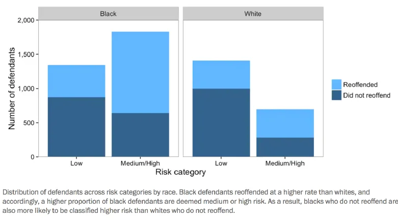
Among defendants who ultimately did not reoffend, black defendants were more than twice as likely as white defendants to be classified as medium or high risk (42 percent vs. 22 percent):

$$P(\text{high risk}\mid \text{not reoffend},\text{black})\gg P(\text{high risk}\mid \text{not reoffend},\text{white}).$$

Even though these defendants did not commit a crime, the black ones are treated more harshly by the courts.

Slides 11-14: defendants per risk category and race, split into reoffended (light) and did not reoffend (dark).

Where the two views come from, read off the figure:

• Fair: within each risk category the proportion of defendants who reoffend is about the same for both groups (the “low” bars have about the same light/dark ratio for black and white, and so do the “medium/high” bars). That is a statement conditioned on the score.
• Unfair: for black defendants the two dark areas (did not reoffend) in “low” and “medium/high” are nearly the same size; for white defendants they are not. Black defendants who don’t reoffend are predicted riskier. That is a statement conditioned on the true outcome.
• Why both can happen: in the raw data black defendants reoffend at a higher rate than white defendants. A classifier that is perfect in terms of accuracy classifies black defendants as medium or high risk more often (58 percent vs. 33 percent).

So who is right?

It depends on how we measure fairness and how we measure the “success” of the system. For this data it is impossible to construct a non-trivial classifier that is fair with respect to both points of view. (Sources: Angwin, Larson, Mattu and Kirchner, “Machine bias”, ProPublica 2016; Washington Post, 2016.)

Side remark: the data has more obvious problems. Some released people reoffended but were never caught, and the chance of that may depend, for example, on where they live. This introduces further bias (measurement vs. construct, Lecture 7).

Example: college admission and affirmative action

Slides 17-20

Harvard admissions lawsuit (2014/15): students complained that the admission rules are unfair. An Asian-American male applicant, not disadvantaged, with a 25% chance of admission would have 36% as a white applicant, 77% as Hispanic and 95% as African-American, all other characteristics the same:

$$\begin{array}{rl}P(\text{accepted}\mid f,\text{asian-am.})& \ll P(\text{accepted}\mid f,\text{white})\\ & \ll P(\text{accepted}\mid f,\text{hispanic})\\ & \ll P(\text{accepted}\mid f,\text{african-am.}).\end{array}$$

Is this obviously unfair? The reason is affirmative action. Harvard: dropping race as one factor would give a class that “fails to achieve the diversity and excellence that Harvard seeks”. In October 2019 the judges concluded that Harvard’s practice was lawful: race may act as a “plus” or “tip”; there are no workable race-neutral alternatives; under the court’s preferred model there is no statistically significant difference between similarly situated Asian-American and white applicants. (Sources: admissionscase.harvard.edu, potentially biased; fairml book, section on counterfactual discrimination analysis.)

More examples

Slides 21-27

• Credit scoring: in a linear model predicting whether applicants pay back a credit, the ZIP code turns out to be a very strong predictor. Living in a low-income neighborhood makes it harder to get credit; you have to “compensate” with, say, a higher income.
• Deliveries: Amazon chose the neighborhoods for free same-day delivery with a data-driven system. A 2016 study found that in many US cities white residents were more than twice as likely as black residents to live in a qualifying neighborhood.
• Street Bump: a Boston app detects potholes with smartphone sensors and reports them to the city. Areas with many elderly people, and low-income neighborhoods, have fewer smartphones, so their streets get reported and fixed less.
• Recruiting (Amazon): about 10 years ago Amazon (74 percent of managerial positions held by men) used a tool to screen applications, trained on 10 years of resumes, predominantly from white males. It penalized resumes containing the word “women” and downgraded graduates of women’s colleges; it was discontinued (Business Insider 2018; Brookings).
• Recruiting (Austria): the employment agency planned to classify unemployed persons into “low”, “middle”, “high” chances of finding a job (features: age, education, prior jobs) and to spend more effort on the top group. Criticism: it can turn existing discrimination into a technical solution; female gender and older age provably lead to a worse evaluation (Süddeutsche Zeitung, 2019).
• Word embeddings (word2vec) map words to ${\mathbb{R}}^{300}$ and support word arithmetic: “London is to England as Paris is to France”, $r(\text{England})+r(\text{Paris})-r(\text{France})\approx r(\text{London})$ (the slide writes the difference $r(\text{France})-r(\text{Paris})$, the sign has to be the other way round). Asking “man is to X as woman is to Y” gives computer programmer / homemaker, surgeon / nurse, brilliant / lovely: the embedding reproduces the gender stereotypes of the text corpus (Bolukbasi et al., NeurIPS 2016).

First take-away

Slides 28-30

What the examples show

• All kinds of biases can happen implicitly in automatic systems. Mostly the designers did not intend to discriminate (Street Bump, word embeddings); some intentionally promoted minorities (affirmative action).
• There is no unique definition of fairness. Many definitions exist, and they typically exclude each other. Which one is appropriate differs between applications and must be discussed in the context of society.
• A “fair” system may have to give up performance elsewhere: overall accuracy (COMPAS) or utility and profit (credit scoring).
• Fairness as a criterion is a request that comes from society. It is hard to find a real application of ML without potentially discriminatory behavior: this is an issue, always, and typically there is no simple solution.

Sources of unfairness

Slides 31-35

• Minorities: a model with 5% overall error can perform terribly on a minority group. Minorities get “drowned” in systems that maximize accuracy, because the training and test error barely change when the minority is misclassified. Worse, minorities are often under-represented relative to the population (sampling bias).
• Biases in data. Sampling bias: demographic, geographic, behavioral or temporal biases in data collection. Example: crime records only contain crimes observed by the police; more officers go where the recorded crime rate was high, so more crimes are recorded there, even if other regions later have more crime. Pre-existing biases: gender roles in text and images, racial stereotypes, past hiring data, word embeddings.
• Measurement of features: which features we measure, and how, shapes the model and can systematically favor or disfavor groups.
• Target variable: the target in social contexts is often a coarse proxy for what we want to measure; by choosing it we already encode biases (the measurement section of Lecture 7).

Discussion

Fairness is not a technical requirement but one that comes from society. Nothing about fairness is obvious and simple.

Basic notions of fairness

Setup

Slides 37-38

There is no unique definition; below are popular ones, many more exist.

Data for group fairness

• Features $X\in \mathcal{X}$.
• Protected / sensitive attribute $A\in \mathcal{A}$ (gender, race, …); depending on the application it is explicitly known or not.
• True target $Y\in \mathcal{Y}$.
• A classifier $C:\mathcal{X}\times \mathcal{A}\to \mathcal{Y}$ predicts $\hat{Y}$ (an estimate of $Y$, or something more abstract).

For simplicity everything is binary: $A$ (black / white), $Y$ (“reoffends or not”), $\hat{Y}$ (“kept in jail / released on bail”).

Demographic parity (independence)

Slides 39-41

Demographic parity (called independence in the fairml book)

$$P(\hat{Y}=1\mid A=1)=P(\hat{Y}=1\mid A=0).$$

Independently of all other features, both groups have the same rate of success. General form beyond the discrete case: $\hat{Y}\perp A$.

Examples: the same proportion of males ($A=0$) and females ($A=1$) is promoted ($\hat{Y}=1$); the same proportion of white and black people is released on bail.

Demographic parity is very strong

It forbids any dependence between the decision and $A$. As soon as the true target $Y$ is correlated with $A$, this can be highly problematic. Example (own): a disease that is twice as common in group $A=1$. Demographic parity forces a screening test to flag both groups equally often, so it must either miss sick people in group 1 or flag healthy people in group 0. Even a perfect classifier violates it.

Equalized odds (separation)

Slides 42-44

Equalized odds (called separation in the fairml book)

All groups have the same false negative rate and the same false positive rate:

$$\begin{array}{rl}P(\hat{Y}=0\mid Y=1,A=0)& =P(\hat{Y}=0\mid Y=1,A=1)\text{and}\\ P(\hat{Y}=1\mid Y=0,A=0)& =P(\hat{Y}=1\mid Y=0,A=1).\end{array}$$

General form: $\hat{Y}\perp A\mid Y$. If one direction matters more, one can require just one of the two; requiring equal true positive rates (equivalently equal false negative rates) is called equal opportunity (Hardt, Price, Srebro 2016).

Examples: among students who have the potential to achieve an MSc degree ($Y=1$), the probability to be accepted ($\hat{Y}=1$) is the same for male and female applicants. Among people who do not reoffend, the probability to be released on bail is the same for white and black defendants.

Sounds good. But: the perfect classifier (false negative and false positive rate 0) is always perfectly fair under this definition. Hm…

Recap: conditional independence

For discrete random variables, $A\perp B\mid C$ iff

$$P(A=a,B=b\mid C=c)=P(A=a\mid C=c)\cdot P(B=b\mid C=c),$$

equivalently $P(A=a\mid B=b,C=c)=P(A=a\mid C=c)$. In words: once $C$ is known, knowing $B$ gives no further information about $A$.

Memory aid

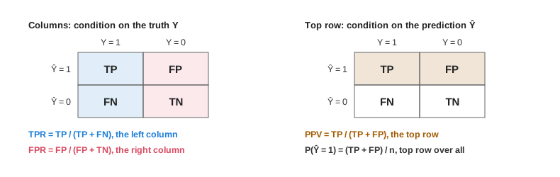
Columns = truth. Equalized odds: people with the same true label get the same treatment in both groups. Predictive parity looks along the rows (same prediction).

Predictive parity (sufficiency) and calibration

Slides 45-46

Predictive parity (called sufficiency in the fairml book)

$$\forall y:P(Y=1\mid \hat{Y}=y,A=0)=P(Y=1\mid \hat{Y}=y,A=1).$$

If the prediction for a person is $\hat{Y}=y$, the probability that truly $Y=1$ is the same for all groups. General form: $Y\perp A\mid \hat{Y}$.

This is the first COMPAS point of view: for a predicted score $\hat{y}\in \{1,\dots ,10\}$ the probability to reoffend is the same for black and white defendants, so a judge who sees $\hat{y}$ can treat both the same.

Calibration by group

If the score is meant to predict a probability (of reoffending, say), it is calibrated by group if for all score values $y$ and groups $a$

$$P(Y=1\mid \hat{Y}=y,A=a)=y.$$

The probabilities are “correct”. In simple cases calibration and predictive parity are more or less the same, but not always (fairml book; Chouldechova, “Fair prediction with disparate impact”, 2017).

Which variable do you condition on?

criterion	conditions on	rate	in the table
demographic parity	nothing (only $A$)	$P(\hat{Y}=1\mid A)$	(TP + FP) / n
equalized odds	the true label $Y$	TPR $=P(\hat{Y}=1\mid Y=1,A)$, FPR $=P(\hat{Y}=1\mid Y=0,A)$	TP / (TP + FN), FP / (FP + TN): columns
predictive parity	the prediction $\hat{Y}$	PPV $=P(Y=1\mid \hat{Y}=1,A)$	TP / (TP + FP): rows

Writing the TPR as $P(\hat{Y}=1\mid \dots )$ with $\hat{Y}$ behind the bar, or dividing TP by TP + FP, computes the PPV instead. That was a real exam mistake.

Extreme cases

Slides 47-48

For binary classification with a binary sensitive attribute:

• Constant classifier $\hat{Y}=1$ for all inputs: the output is independent of everything, in particular of $A$. It is maximally fair: it satisfies demographic parity and equalized odds (both TPR and FPR are 1 in both groups).
• Predicting the sensitive attribute, $\hat{Y}=1⟺A=1$: the output is identical to $A$, maximally unfair with respect to demographic parity and equalized odds.

Impossibility results

Criteria that cannot hold together

Slides 49-52

In non-trivial situations the criteria typically cannot hold at the same time (fairml book; Kleinberg, Mullainathan, Raghavan, “Inherent trade-offs in the fair determination of risk scores”, 2016).

Proposition (demographic parity vs. predictive parity)

Assume all events of the joint distribution of $(A,\hat{Y},Y)$ have positive probability and $A$ and $Y$ are not independent. Then demographic parity and predictive parity cannot both hold.

Proof

$$\begin{array}{rlrl}P(A=a,Y=y,\hat{Y}=\hat{y})& =P(A=a\mid Y=y,\hat{Y}=\hat{y})P(Y=y,\hat{Y}=\hat{y})& & \\ & =P(A=a\mid \hat{Y}=\hat{y})P(Y=y,\hat{Y}=\hat{y})& & \text{(predictive parity: }Y\perp A\mid \hat{Y})\\ & =P(A=a)P(Y=y,\hat{Y}=\hat{y})& & \text{(demographic parity: }\hat{Y}\perp A)\end{array}$$

So $A\perp (Y,\hat{Y})$, which implies $A\perp Y$: a contradiction to the assumption. $\square$

Proposition (equalized odds vs. predictive parity)

Under the same assumptions ($A$ not independent of $Y$), equalized odds and predictive parity cannot both hold. Proof: by similar arguments, $A\perp \hat{Y}\mid Y$ and $A\perp Y\mid \hat{Y}$ imply $A\perp (Y,\hat{Y})$, hence $A\perp Y$, a contradiction.

A third version: if $Y$ is binary, $A$ is not independent of $Y$ and $\hat{Y}$ is not independent of $Y$, then demographic parity and predictive parity cannot both hold (elementary, proof skipped).

In words

When the base rates $P(Y=1\mid A=a)$ differ between groups, you have to choose which criterion to give up. COMPAS: calibrated scores (predictive parity) and equal error rates (equalized odds) are incompatible because black and white defendants reoffend at different rates in the data.

Memory aid

Different base rates → pick your fairness. Calibrated scores and equal error rates cannot both hold (COMPAS).

Task: extreme classifiers and base rates

Exam-style task: which criteria hold? (4 P)

Math: (conditional) independence

Group $A=0$ has 80 of 200 people with $Y=1$, group $A=1$ has 50 of 100.

(a) (1 P, easy) The constant classifier $\hat{Y}=1$: which of demographic parity, equalized odds, predictive parity hold?

(b) (1.5 P, harder) The perfect classifier $\hat{Y}=Y$: which hold?

(c) (1.5 P, transfer) Explain with the propositions why no classifier can satisfy demographic parity and predictive parity here. What would change if both groups had 40% positives?

Solution

(a) DP: $P(\hat{Y}=1\mid A)=1$ in both groups, holds. Equalized odds: TPR $=1$ and FPR $=1$ in both, holds. Predictive parity: $P(Y=1\mid \hat{Y}=1,A)$ is the base rate, $0.4$ vs. $0.5$, violated. (1 P)

(b) DP: $P(\hat{Y}=1\mid A)$ is the base rate, $0.4$ vs. $0.5$, violated. Equalized odds: TPR $=1$, FPR $=0$ in both, holds. Predictive parity: $P(Y=1\mid \hat{Y}=1,A)=1$ and $P(Y=1\mid \hat{Y}=0,A)=0$ in both, holds. (1.5 P)

(c) The base rates differ, so $A$ and $Y$ are dependent. If DP ($\hat{Y}\perp A$) and PP ($Y\perp A\mid \hat{Y}$) both held, then $P(a,y,\hat{y})=P(a)P(y,\hat{y})$, so $A\perp Y$: contradiction. With equal base rates $A\perp Y$ is possible and the propositions no longer apply; e.g. the perfect classifier would then satisfy all three criteria. (1.5 P)

Individual and counterfactual fairness

Slides 53-54

• Individual fairness (Dwork, Hardt, Pitassi, Reingold, Zemel, “Fairness through awareness”, 2012): not about groups but individuals. Two individuals who are “similar” according to a pre-specified metric should receive similar treatment. Hard to use in practice: what is the right notion of similarity, in the input space and in the target space?
• Counterfactual fairness (Russell, Kusner, Loftus, Silva, NeurIPS 2017): with a causal model, compute what (the distribution of) a variable would have been had other variables been different, all else equal. Example: “Would individual $i$ have graduated ($Y=1$) if they hadn’t had a job?”

Lots of criteria

Slides 55-56

Many criteria exist and have been invented several times. The fairml book matches each to its closest relative among the three (no need to memorize the names):

closest relative	criteria (equivalent or a relaxation)
independence ($\hat{Y}\perp A$)	statistical parity, group fairness, demographic parity, conditional statistical parity, Darlington criterion (4)
separation ($\hat{Y}\perp A\mid Y$)	equal opportunity, equalized odds, conditional procedure accuracy, avoiding disparate mistreatment, balance for the negative class, balance for the positive class, predictive equality, equalized correlations, Darlington criterion (3)
sufficiency ($Y\perp A\mid \hat{Y}$)	Cleary model, conditional use accuracy, predictive parity, calibration within groups, Darlington criterion (1), (2)

Lots of criteria, no single one

• The one, unique fairness criterion does not exist.
• Fairness comes from society and cannot always be captured satisfactorily by statistical definitions.
• All existing criteria are plausible in some applications, but all have serious drawbacks and miss important aspects (see the fairml book).
• But also: the baseline is decisions made by humans, and they are definitely biased as well.

Technical approaches to improve fairness

Three approaches

Slide 58

Pre-, in- and post-processing

• Pre-processing: try to fix the bias in the data.
• Training (in-processing): learn decisions that are accurate and fair at the same time.
• Post-processing: fix an unfair black-box model in hindsight.

Fixing unfairness in the data

Slides 59-61

First naive idea: remove the sensitive features. This is pretty much impossible, because many other variables are highly correlated with the sensitive attribute and the algorithm uses them as proxies. Standard example: in many cities some quarters are predominantly white or black, and often the black population has a low income. The ZIP code is then correlated with both income and race, and it may be harder to get credit in those quarters. Even if race is not a feature, it is implicitly present whenever the ZIP code is used. (This is Sheet 11, Exercise 2.)

• In many cases the discriminatory features are not even well defined. Some patterns (smoking is associated with cancer) are knowledge we want to mine, others (girls like pink, boys like blue) are stereotypes we want to avoid. It is hard (impossible) to tell the algorithm which patterns to find, and humans may not agree either.
• Removing all variables correlated with the sensitive attribute often removes all relevant variables, in particular with several sensitive variables (gender and race). And sometimes the sensitive attribute is not even available, so the correlations cannot be computed.

Training for accuracy and fairness

Slides 62-64

Standard setup: minimize the empirical risk ${\hat{R}}_n(f)$ over $\mathcal{F}$, with a regularizer $\Omega (f)$ (Lecture 5). Two groups $A\in \{0,1\}$, target: demographic parity. The true unfairness is the demographic parity difference, and its empirical version uses the group sizes $n_1,n_0$:

$$\mathrm{unf}(f)=|P(f(x)>0\mid A=1)-P(f(x)>0\mid A=0)|,$$ $$\widehat{\mathrm{unf}}(f)=|\frac{1}{n_1}\sum _{i:a_i=1}{1}_{f(x_i)>0}-\frac{1}{n_0}\sum _{i:a_i=0}{1}_{f(x_i)>0}|.$$

The fair learning problem:

$$\underset{f\in \mathcal{F}}{\min }{\hat{R}}_n(f)+\lambda \Omega (f)\text{subject to}\widehat{\mathrm{unf}}(f)<\tau .$$

Easy or difficult?

• $\widehat{\mathrm{unf}}$ is discrete (indicator functions), so it is hard to optimize, like the 0-1 loss (surrogate losses).
• Standard solution: convex relaxations. But most existing relaxations are too loose: even if the relaxed fairness is perfectly satisfied, the true fairness can be very bad (Lohaus, Perrot, von Luxburg, “Too relaxed to be fair”, 2020; Zafar, Valera, Rodriguez, Gummadi, “Fairness constraints”, 2017).
• The lecturer’s view: this approach is the most useful one, but currently nothing out there works really well.

Fixing models in hindsight

Slides 65-68

Scenario: an agency or company trains a classifier privately (credit assessment, COMPAS). Someone evaluates it and finds it unfair. Can we fix it without access to its internals? We only see the prediction $\hat{Y}$ and the sensitive attribute $A$ (needed for the evaluation). All we can do is build a derived classifier that takes $\hat{Y}$ and $A$ as input and outputs a new, possibly randomized, $\tilde{Y}$.

Derived classifier (binary $\hat{Y}$ and $A$)

Exactly four parameters:

$$p_{ya}=P(\tilde{Y}=1\mid \hat{Y}=y,A=a),y\in \{0,1\},a\in \{0,1\}.$$

Then for each group

$$\begin{array}{rl}{\mathrm{TPR}}_a(\tilde{Y})& =p_{1a}{\mathrm{TPR}}_a+p_{0a}(1-{\mathrm{TPR}}_a),\\ {\mathrm{FPR}}_a(\tilde{Y})& =p_{1a}{\mathrm{FPR}}_a+p_{0a}(1-{\mathrm{FPR}}_a).\end{array}$$

The $p_{ya}$ can be chosen (by a linear program) so that $\tilde{Y}$ satisfies equal opportunity or equalized odds. Randomization helps to get a better accuracy-fairness tradeoff, but accuracy may still decrease; Hardt, Price and Srebro (NeurIPS 2016) give guarantees.

The reachable $(\mathrm{FPR},\mathrm{TPR})$ points of group $a$ form the quadrilateral with corners $(0,0)$, $(1,1)$, $({\mathrm{FPR}}_a,{\mathrm{TPR}}_a)$ and $(1-{\mathrm{FPR}}_a,1-{\mathrm{TPR}}_a)$ (keep, never predict 1, always predict 1, flip). Equalized odds needs a point both groups can reach.

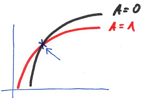
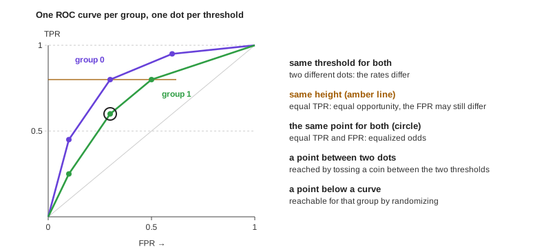
With a score: if we see a real-valued score $f(X)$ that is thresholded, $\hat{Y}=1⟺f(X)\ge t$, plot the ROC curves of both groups separately and choose the point where they intersect (with group-specific thresholds). There both groups have the same false positive and false negative rates. If the curves do not intersect, a randomized predictor still solves it.

Slides 67-68: ROC curves of the two groups; at the intersection both have the same TPR and FPR.

Task: fairness from two tables

Exam-style task: two group tables (4 P)

Math: conditional probability in a table

A loan screening model is evaluated separately for two groups ($Y=1$: pays back, $\hat{Y}=1$: loan granted).

$A=0$	$Y=1$	$Y=0$
$\hat{Y}=1$	60	24
$\hat{Y}=0$	20	96

$A=1$	$Y=1$	$Y=0$
$\hat{Y}=1$	30	5
$\hat{Y}=0$	20	45

(a) (1 P, easy) Compute $P(\hat{Y}=1\mid A=a)$ for both groups. Does demographic parity hold?

(b) (1.5 P, harder) Compute TPR and FPR for both groups. Does equal opportunity hold? Equalized odds? Compute also $P(Y=1\mid \hat{Y}=1,A=a)$ and explain why this is not the TPR.

(c) (1.5 P, transfer) The bank may only post-process: for each group it chooses $p_{ya}=P(\tilde{Y}=1\mid \hat{Y}=y,A=a)$. Construct a derived classifier with equal opportunity that keeps group 1 unchanged and never grants new loans. What are the new TPR and FPR of group 0, and its accuracy? Does equalized odds hold now?

Solution

(a) $A=0$: $(60+24)/200=0.42$. $A=1$: $(30+5)/100=0.35$. $0.42\ne 0.35$: demographic parity is violated. (1 P)

(b) Condition on the true label (columns). $A=0$: TPR $=60/80=0.75$, FPR $=24/120=0.2$. $A=1$: TPR $=30/50=0.6$, FPR $=5/50=0.1$. TPRs differ, so neither equal opportunity nor equalized odds holds. $P(Y=1\mid \hat{Y}=1,A=0)=60/84\approx 0.714$ and $30/35\approx 0.857$ for $A=1$: this is the PPV, conditioned on the prediction (a row), not on the true label. (1.5 P)

(c) Lower the higher TPR: $p_{10}=q$, $p_{00}=0$, and $p_{11}=1$, $p_{01}=0$ for group 1. New TPR of group 0: $0.75q=0.6\Rightarrow q=0.8$ (each granted loan in group 0 is kept with probability 0.8). New FPR: $0.2\cdot 0.8=0.16$. Expected counts in group 0: TP $48$, FN $32$, FP $19.2$, TN $100.8$, accuracy $(48+100.8)/200=0.744$ (before $0.78$). Equal opportunity holds (0.6 = 0.6), equalized odds does not (FPR 0.16 vs. 0.1). The fairness costs accuracy, and the decision is now randomized. (1.5 P)

Practice: fairness from two tables

Edit the counts of both tables; all rates and the four criteria update. Hover a metric to see which cells it uses. Random practice tables hide the results until you uncheck the box. Below: the derived classifier of the post-processing, its reachable region per group on the ROC plane, and buttons for equal opportunity and equalized odds.

With the task numbers: “equal opportunity: lower the higher TPR” reproduces (c). “Raise the lower TPR” instead flips 37.5% of group 1’s rejections to approvals and pushes its FPR to 0.44. “Equalized odds” finds the most accurate point that both groups can reach, here FPR 0.168 and TPR 0.630: both groups must move.

Task: thresholds on ROC curves

Exam-style task: group thresholds (4 P)

A score is thresholded at $t_1>t_2>t_3$. The resulting (FPR, TPR) points per group:

threshold	$A=0$	$A=1$
$t_1$	(0.10, 0.50)	(0.05, 0.30)
$t_2$	(0.20, 0.70)	(0.10, 0.50)
$t_3$	(0.40, 0.90)	(0.25, 0.70)

(a) (1 P, easy) With one common threshold $t_2$: does equal opportunity hold?

(b) (1.5 P, harder) Find group-specific thresholds with equalized odds, and ones with equal opportunity at TPR $0.7$. Does the second choice also give equalized odds?

(c) (1.5 P, transfer) Name two objections against group-specific thresholds or randomized post-processing in a bail decision.

Solution

(a) TPR $0.70$ vs. $0.50$: no. (1 P)

(b) $A=0$ at $t_1$ and $A=1$ at $t_2$: both $(0.10,0.50)$, equalized odds holds (the ROC points coincide). TPR $0.7$: $A=0$ at $t_2$, $A=1$ at $t_3$, equal opportunity holds, but FPR $0.20$ vs. $0.25$, so no equalized odds. (1.5 P)

(c) Group-specific thresholds use the sensitive attribute explicitly at decision time (two people with the same score get different decisions), which may be illegal or perceived as unfair to individuals. Randomization means that the outcome for an individual depends on a coin flip (who stays in jail?). Also: accuracy decreases, and the fix does not address biased data or target variables. (1.5 P)

Tradeoffs

Accuracy, randomization and feedback loops

Slides 70-74

• Accuracy vs. fairness: fair classifiers optimize two objectives. The accuracy of a fair classifier can only be $\le$ that of the classifier optimized for accuracy alone. A choice has to be made: how much accuracy loss do we tolerate for how much fairness?
• Fair classifiers can require randomization: especially when classifiers are modified in hindsight, it is often impossible to reach fairness without randomization (Agarwal, Beygelzimer, Dudík, Langford, Wallach, “A reductions approach to fair classification”, 2018; Hardt, Price, Srebro 2016). Depending on the application this is highly questionable: a randomized decision about who stays in jail?
• Feedback loops. Self-fulfilling predictions: a predictive policing system marks some areas as high risk, more officers are sent there, more crimes are detected there, and the prediction appears validated even if the risk is not higher. Predictions that affect the training set: the resulting arrests are added to the training data, so the areas keep looking risky (Ensign, Friedler, Neville, Scheidegger, Venkatasubramanian, “Runaway feedback loops in predictive policing”, 2017).

Discussion

Fairness has a long history of debate in ethics, sociology and many other fields. From the data and from the negative theoretical results: there often is no obvious “solution”. In practice many decisions must be taken (which notion of fairness, which tradeoff, is randomization acceptable, …), and different decisions lead to different solutions. Most of these issues cannot be fixed by technical solutions. Society has to decide (but we need to help and explain the issues). See also Corbett-Davies and Goel, “The measure and mismeasure of fairness”, 2018.

Summary

Topic	Key message
COMPAS	calibrated per score (fair) but unequal false positive rates (unfair); with different base rates both cannot hold
sources	minorities drown in accuracy, sampling bias, pre-existing bias, feature and target choice
demographic parity	$\hat{Y}\perp A$: equal $P(\hat{Y}=1\mid A)$; the constant classifier satisfies it, the perfect one may not
equalized odds	$\hat{Y}\perp A\mid Y$: equal TPR and FPR (columns); equal opportunity = equal TPR; the perfect classifier satisfies it
predictive parity	$Y\perp A\mid \hat{Y}$: equal $P(Y=1\mid \hat{Y},A)$ (rows); calibration $P(Y=1\mid \hat{Y}=y,A)=y$
impossibility	$A/\perp Y$: not DP and PP together, not EO and PP together
other notions	individual fairness (similar people, similar treatment), counterfactual fairness (causal model)
fixes	removing $A$ fails (proxies); constrained training (loose relaxations); post-processing with $p_{ya}$ or ROC intersection, often randomized
tradeoffs	accuracy loss, randomization, feedback loops; society decides

Self-Test

Question cards (12)

Explain the two views in the COMPAS debate. Which fairness criterion does each correspond to?

Answer

Northpointe: for each score the reoffending rate is the same for black and white defendants, i.e. predictive parity / calibration ($Y\perp A\mid \hat{Y}$). ProPublica: among non-reoffenders, black defendants get high scores far more often (42% vs. 22%), i.e. unequal false positive rates, a violation of equalized odds.

Why can both COMPAS views be right at the same time?

Answer

The base rates differ (black defendants reoffend more often in the data). With $A/\perp Y$, equalized odds and predictive parity cannot both hold, so a calibrated score necessarily has unequal error rates.

Define demographic parity, equalized odds and predictive parity for binary variables, and as independence statements.

Answer

DP: $P(\hat{Y}=1\mid A=0)=P(\hat{Y}=1\mid A=1)$, $\hat{Y}\perp A$. EO: equal FNR $P(\hat{Y}=0\mid Y=1,A)$ and FPR $P(\hat{Y}=1\mid Y=0,A)$, $\hat{Y}\perp A\mid Y$. PP: $P(Y=1\mid \hat{Y}=y,A=0)=P(Y=1\mid \hat{Y}=y,A=1)$ for all $y$, $Y\perp A\mid \hat{Y}$.

What is the difference between the TPR and the PPV? How do you read them off a confusion table?

Answer

TPR $=P(\hat{Y}=1\mid Y=1)=\mathrm{TP}/(\mathrm{TP}+\mathrm{FN})$, conditioned on the true label (column). PPV $=P(Y=1\mid \hat{Y}=1)=\mathrm{TP}/(\mathrm{TP}+\mathrm{FP})$, conditioned on the prediction (row). Equalized odds uses TPR/FPR, predictive parity uses PPV.

Why is demographic parity problematic when $Y$ depends on $A$?

Answer

It forces equal positive rates although the true rates differ, so even the perfect classifier violates it; satisfying it means misclassifying people in at least one group on purpose.

Which criteria do the constant classifier and the perfect classifier satisfy?

Answer

Constant $\hat{Y}=1$: demographic parity and equalized odds (TPR = FPR = 1), not predictive parity if base rates differ. Perfect $\hat{Y}=Y$: equalized odds and predictive parity, not demographic parity if base rates differ.

Prove that demographic parity and predictive parity cannot both hold if $A$ and $Y$ are dependent.

Answer

$P(a,y,\hat{y})=P(a\mid y,\hat{y})P(y,\hat{y})=P(a\mid \hat{y})P(y,\hat{y})$ (PP) $=P(a)P(y,\hat{y})$ (DP). So $A\perp (Y,\hat{Y})$, hence $A\perp Y$: contradiction.

Name the sources of unfairness from the lecture.

Answer

Minorities drowned in accuracy maximization and under-represented; sampling bias (crime records reflect police presence); pre-existing biases (stereotypes, past hiring); choice and measurement of features; target variable as a proxy for the construct.

Why does removing the sensitive attribute not make a classifier fair?

Answer

Other features are correlated with it and act as proxies (ZIP code for race and income). Removing all correlated features removes most relevant information, and the attribute may be unavailable to even compute correlations.

What is the problem with training under a fairness constraint $\widehat{\mathrm{unf}}(f)<\tau$?

Answer

The constraint consists of indicator functions, so it is discrete and hard to optimize. Convex relaxations are used, but most are too loose: the relaxed constraint can hold while the true unfairness is large.

How does post-processing with a derived classifier work, and why is it randomized?

Answer

Only $\hat{Y}$ and $A$ are used: choose $p_{ya}=P(\tilde{Y}=1\mid \hat{Y}=y,A=a)$ so that the new TPR/FPR match across groups. Matching an intermediate rate requires keeping or flipping predictions with a probability strictly between 0 and 1, so decisions become random.

What is a feedback loop in predictive policing?

Answer

Areas predicted as risky get more police, so more crimes are recorded there; the prediction seems confirmed and the new arrests enter the training data, so the areas keep being predicted risky even without a higher true crime rate.

Multiple Choice

Multiple choice (7)

Group $A=0$: TP 40, FN 10, FP 20, TN 30. What is the TPR of group 0?

• $40/60\approx 0.67$

• $40/50=0.8$

• $60/100=0.6$

• $20/50=0.4$

Explanation

TPR $=P(\hat{Y}=1\mid Y=1)=\mathrm{TP}/(\mathrm{TP}+\mathrm{FN})$. $40/60$ is the PPV, $0.6$ the positive prediction rate, $0.4$ the FPR.

Equalized odds requires

• $\hat{Y}\perp A$

• $\hat{Y}\perp A\mid Y$

• $Y\perp A\mid \hat{Y}$

• $Y\perp A$

Explanation

Separation: equal TPR and FPR across groups. $\hat{Y}\perp A$ is demographic parity, $Y\perp A\mid \hat{Y}$ predictive parity.

The COMPAS score has about the same reoffending rate per score value in both groups. This is

• demographic parity

• equal opportunity

• predictive parity (calibration by group)

• individual fairness

Explanation

Conditioning on the score (prediction) and comparing the true outcome rate is sufficiency / predictive parity.

Which classifier always satisfies equalized odds?

• the classifier that predicts the sensitive attribute

• the perfect classifier $\hat{Y}=Y$

• any calibrated classifier

• any classifier that does not use $A$ as a feature

Explanation

TPR = 1 and FPR = 0 in all groups. Not using $A$ does not help because of proxies; calibration conflicts with equalized odds when base rates differ.

Two groups have different base rates $P(Y=1\mid A)$. Which pair of criteria can a non-trivial classifier NOT satisfy simultaneously?

• equal opportunity and equalized odds

• equalized odds and predictive parity

• equal opportunity and equal FNR

• demographic parity and the use of randomization

Explanation

Proposition on slide 51. Equal opportunity is part of equalized odds, and equal TPR is the same as equal FNR.

A post-processing step keeps each positive prediction in group 0 with probability 0.8, and the old TPR of group 0 was 0.9. The new TPR is

• 0.9

• 0.8

• 0.72

• 0.1

Explanation

$p_{1,0}\mathrm{TPR}+p_{0,0}(1-\mathrm{TPR})=0.8\cdot 0.9+0=0.72$.

Why does removing the feature "race" usually not remove racial bias?

• Because the model memorizes the removed feature.

• Because correlated features such as the ZIP code act as proxies.

• Because demographic parity requires the feature.

• Because training data always contains race explicitly.

Explanation

Slide 59: race is implicitly present whenever correlated variables are used.

Cheat sheet and full integration tasks

The two tasks below use every calculation of this lecture once: the rates and criteria from two group tables with randomized post-processing, then thresholds on ROC points. Write your own sheet first, solve the tasks with it next to you, then open the sheet at the bottom and compare. The letters in brackets name the block of the sheet that a subtask needs.

Full integration task: two group tables (16 P)

Math: conditional probability in a table

A hiring model is evaluated separately for two groups ($Y=1$: suitable, $\hat{Y}=1$: invited).

$A=0$	$Y=1$	$Y=0$
$\hat{Y}=1$	120	60
$\hat{Y}=0$	40	180

$A=1$	$Y=1$	$Y=0$
$\hat{Y}=1$	50	20
$\hat{Y}=0$	50	80

(a) (2 P, blocks A and B) Compute $P(\hat{Y}=1\mid A=a)$ for both groups. Does demographic parity hold?

(b) (3 P, blocks A and B) Compute TPR and FPR for both groups. Does equal opportunity hold? Equalized odds?

(c) (2 P, blocks A and B) Compute $P(Y=1\mid \hat{Y}=1,A=a)$ and the base rates $P(Y=1\mid A=a)$. Does predictive parity hold for $\hat{Y}=1$? Why is this number not the TPR?

(d) (4 P, block C) Only post-processing is allowed: $p_{ya}=P(\tilde{Y}=1\mid \hat{Y}=y,A=a)$. Reach equal opportunity by lowering the higher TPR, without new invitations. Give the $p_{ya}$, the new TPR, FPR, expected counts and accuracy of the changed group. Does equalized odds hold now?

(e) (3 P, block C) Reach equal opportunity the other way: raise the lower TPR and never withdraw an invitation. Give the $p_{ya}$, the new FPR and accuracy of the changed group, and compare with (d).

(f) (2 P, block B) Can any classifier satisfy demographic parity and predictive parity on this population? Which of the three criteria does the perfect classifier $\hat{Y}=Y$ satisfy here?

Solution

(a) $A=0$: $(120+60)/400=0.45$. $A=1$: $(50+20)/200=0.35$. Demographic parity is violated. (2 P)

(b) Condition on the true label, that is read the columns. $A=0$: TPR $=120/160=0.75$, FPR $=60/240=0.25$. $A=1$: TPR $=50/100=0.5$, FPR $=20/100=0.2$. The TPRs differ, so equal opportunity fails, and with it equalized odds. (3 P)

(c) Read the top row: $A=0$: $120/180\approx 0.67$. $A=1$: $50/70\approx 0.71$. Not equal, predictive parity fails. Base rates: $160/400=0.4$ and $100/200=0.5$. The number is the PPV: it conditions on the prediction (a row). The TPR conditions on the truth (a column). (2 P)

(d) Group 0 has the higher TPR. Keep each of its invitations with probability $q$: $p_{10}=q$, $p_{00}=0$, and group 1 unchanged, $p_{11}=1$, $p_{01}=0$. $0.75q=0.5\Rightarrow q=\frac{2}{3}$. New FPR of group 0: $0.25\cdot \frac{2}{3}\approx 0.167$. Expected counts: TP $=80$, FN $=80$, FP $=40$, TN $=200$. Accuracy $280/400=0.70$, before $0.75$. Equal opportunity holds ($0.5=0.5$). Equalized odds does not: FPR $0.167$ against $0.2$. (4 P)

(e) Group 1 has the lower TPR. Keep its invitations and invite a rejected person with probability $q$: $p_{11}=1$, $p_{01}=q$. $0.5+q(1-0.5)=0.75\Rightarrow q=0.5$. New FPR of group 1: $0.2+0.5\cdot 0.8=0.6$. Expected counts: TP $=75$, FN $=25$, FP $=60$, TN $=40$, accuracy $115/200=0.575$, before $0.65$. Both ways reach equal opportunity and both cost accuracy. (d) withdraws invitations from suitable people in group 0, (e) invites 60% of the unsuitable people in group 1. (3 P)

(f) No. The base rates differ ($0.4$ against $0.5$), so $A$ and $Y$ are dependent, and then demographic parity and predictive parity cannot both hold. The perfect classifier has TPR 1 and FPR 0 in both groups, so equalized odds holds, and $P(Y=1\mid \hat{Y}=1)=1$ in both groups, so predictive parity holds. Its invitation rate is the base rate, $0.4$ against $0.5$: demographic parity fails. (2 P)

Full integration task: thresholds on ROC points (6 P)

A score is thresholded at $t_1>t_2>t_3$. The resulting (FPR, TPR) points per group:

threshold	$A=0$	$A=1$
$t_1$	(0.10, 0.40)	(0.05, 0.30)
$t_2$	(0.25, 0.75)	(0.20, 0.50)
$t_3$	(0.50, 0.90)	(0.25, 0.75)

(a) (1 P, block D) With the common threshold $t_2$: does equal opportunity hold?

(b) (2 P, block D) Find group-specific thresholds with equalized odds.

(c) (3 P, block D) Group 0 uses $t_1$. No single threshold gives group 1 the TPR $0.40$. How can group 1 reach it, and which FPR results? Do equal opportunity and equalized odds hold then?

Solution

(a) TPR $0.75$ against $0.50$: no. (1 P)

(b) $A=0$ at $t_2$ and $A=1$ at $t_3$: both at $(0.25,0.75)$. Same TPR and same FPR, so equalized odds holds. (2 P)

(c) Toss a fair coin between $t_1$ and $t_2$ for group 1. The rates are the averages: TPR $=\frac{1}{2}(0.30+0.50)=0.40$ and FPR $=\frac{1}{2}(0.05+0.20)=0.125$. Equal opportunity holds ($0.40=0.40$). Equalized odds does not: FPR $0.125$ against $0.10$. The decision for a person in group 1 now depends on a coin. (3 P)

Cheat sheet: fairness (6 blocks)

A. The table and the rates

Per group, with the truth in the columns and the prediction in the rows:

	$Y=1$	$Y=0$
$\hat{Y}=1$	① TP	② FP
$\hat{Y}=0$	③ FN	④ TN

Rate	From the table	Conditions on
$P(\hat{Y}=1\mid A)$	(① + ②) / $n$	the group only
TPR $=P(\hat{Y}=1\mid Y=1,A)$	① / (① + ③)	the truth: left column
FPR $=P(\hat{Y}=1\mid Y=0,A)$	② / (② + ④)	the truth: right column
PPV $=P(Y=1\mid \hat{Y}=1,A)$	① / (① + ②)	the prediction: top row
base rate $P(Y=1\mid A)$	(① + ③) / $n$	the group only
accuracy	(① + ④) / $n$

Columns are the truth, rows the prediction. TPR and FPR stay inside one column, the PPV stays inside the top row.

B. The criteria

Criterion	Equal in both groups
demographic parity	$P(\hat{Y}=1\mid A)$
equal opportunity	TPR
equalized odds	TPR and FPR
predictive parity	PPV, and $P(Y=1\mid \hat{Y}=0,A)$

You see	It means
the constant classifier $\hat{Y}=1$	demographic parity and equalized odds hold (TPR $=$ FPR $=1$). Predictive parity fails if the base rates differ
the perfect classifier $\hat{Y}=Y$	equalized odds and predictive parity hold. Demographic parity fails if the base rates differ
different base rates	demographic parity and predictive parity cannot both hold. Equalized odds and predictive parity cannot both hold
the sensitive attribute was removed	not enough: other features act as proxies

C. Randomized post-processing

$p_{ya}=P(\tilde{Y}=1\mid \hat{Y}=y,A=a)$. New rates of a group: ${\text{TPR}}^{\prime }=p_1\text{TPR}+p_0(1-\text{TPR})$ and ${\text{FPR}}^{\prime }=p_1\text{FPR}+p_0(1-\text{FPR})$.

Way to equal opportunity	Changed group	Parameters	New FPR
lower the higher TPR	the one with the higher TPR	$p_1=q=\frac{\text{target}}{\text{TPR}}$, $p_0=0$	$q\cdot \text{FPR}$
raise the lower TPR	the one with the lower TPR	$p_1=1$, $p_0=q=\frac{\text{target}-\text{TPR}}{1-\text{TPR}}$	$\text{FPR}+q(1-\text{FPR})$

• New expected counts: TP $=$ TPR${}^{\prime }$ times the positives, FP $=$ FPR${}^{\prime }$ times the negatives. FN and TN are the rest of each column.
• Accuracy $=$ (TP $+$ TN) / $n$. It can only go down.
• Check equalized odds again afterwards: the FPRs usually still differ.

D. ROC points and thresholds

Reading an ROC plot with two groups. Equal height is equal opportunity, the same point is equalized odds.

You see	It means
one common threshold	compare the two points of that row
two thresholds with the same (FPR, TPR)	equalized odds with group-specific thresholds
two thresholds with the same TPR only	equal opportunity, not equalized odds
no threshold hits the wanted rate	mix two thresholds with a coin: the rates are the weighted averages

E. What it costs

You see	It means
a fair classifier	its accuracy is at most that of the unconstrained one
randomized post-processing	the decision for a person depends on a coin
group-specific thresholds	the sensitive attribute is used at decision time: same score, different decision
predictions that change the future data	feedback loop: the prediction confirms itself

F. Traps

• The TPR divides by the actual positives (a column), not by the predicted positives (a row). Dividing TP by TP $+$ FP gives the PPV.
• Read the labels of the table first. If the truth is in the rows, everything above is mirrored.
• Use the numbers of one group for the rates of that group, never the pooled table.
• Equal opportunity is only half of equalized odds.
• Expected counts after randomization need not be whole numbers.

References

All sources cited on the slides, in slide order (19 entries)

Slide	Source	Key point
5, 20, 22, 23, 46, 49, 55	Barocas, Hardt and Narayanan, Fairness and Machine Learning (fairmlbook.org)	textbook, criteria table
15	Angwin, Larson, Mattu and Kirchner, “Machine bias”, ProPublica, 2016	COMPAS unfair view
15	Washington Post, “A computer program used for bail and sentencing decisions was labeled biased against blacks. It’s actually not that clear”, 2016	COMPAS debate
20	Harvard admissions case website	affirmative action ruling
24	Hamilton, “Why it’s totally unsurprising that Amazon’s recruitment AI was biased against women”, Business Insider, 2018	recruiting tool
24	Brookings, “Algorithmic bias detection and mitigation”	recruiting tool
25	Süddeutsche Zeitung, October 2019	Austrian employment agency
27	Bolukbasi, Chang, Zou, Saligrama and Kalai, “Man is to computer programmer as woman is to homemaker? Debiasing word embeddings”, NeurIPS 2016	biased embeddings
46	Chouldechova, “Fair prediction with disparate impact: a study of bias in recidivism prediction instruments”, 2017	calibration
49	Kleinberg, Mullainathan and Raghavan, “Inherent trade-offs in the fair determination of risk scores”, arXiv 1609.05807, 2016	impossibility
53	Dwork, Hardt, Pitassi, Reingold and Zemel, “Fairness through awareness”, 2012	individual fairness
54	Russell, Kusner, Loftus and Silva, “When worlds collide: integrating different counterfactual assumptions in fairness”, NeurIPS 2017	counterfactual fairness
55	criteria table: Darlington 1971; Cleary 1966; Dwork et al. 2011; Corbett-Davies et al. 2017; Berk et al. 2017; Zafar et al. 2017; Woodworth 2017	original criteria
64	Zafar, Valera, Rodriguez and Gummadi, “Fairness constraints: mechanisms for fair classification”, WWW 2017 / ICML 2017	constrained training
64	Lohaus, Perrot and von Luxburg, “Too relaxed to be fair”, 2020	loose relaxations
68, 71	Hardt, Price and Srebro, “Equality of opportunity in supervised learning”, NeurIPS 2016	post-processing, equal opportunity
71	Agarwal, Beygelzimer, Dudík, Langford and Wallach, “A reductions approach to fair classification”, 2018	randomized fair classifiers
73	Ensign, Friedler, Neville, Scheidegger and Venkatasubramanian, “Runaway feedback loops in predictive policing”, arXiv 1706.09847, 2017	feedback loops
74	Corbett-Davies and Goel, “The measure and mismeasure of fairness: a critical review of fair machine learning”, arXiv 2018	review

Related

• Previous: Lecture 8: Overparameterized Learning · Next: Lecture 9.2: Explainability and Law · Course: Overview · Formula Sheet · Glossary
• Concepts: Fairness Criteria, Fair Post-Processing, Measurement and Construct
• Exercises: Sheet 11, Exercise 2 (fairness: removing a feature is not enough)