Lecture 7: Data, Measurement and Validity

TL;DR

1. Measurement: we are interested in a target construct (often not observable) but record a measurement of it. Machine learning does not learn the target construct, it learns the measurement. Examples: health care cost as a proxy for illness (racial bias), 5-year survival as a proxy for life-years gained (young patients lose out).
2. Harms that come with data: under-represented minorities, sampling bias, historically biased patterns, offensive or illegal content, privacy violations (anonymization does not protect), copyright. A model cannot fix flawed data in hindsight: garbage in, garbage out. Good practice: question the measurement, check representativeness, datasheets for datasets.
3. Features: a feature map $\Phi :\mathcal{X}\to {\mathbb{R}}^d$ turns objects into vectors. Non-linear basis functions (polynomial, Fourier, RBF) make linear methods non-linear. Kernels compute $k(x,y)=⟨\Phi (x),\Phi (y)⟩$ without computing $\Phi$ (kernel trick).
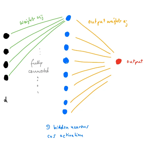
4. Random feature models: draw the parameters of $D$ basis functions at random (random Fourier features $\cos ({\omega }_j^{\top }x+b_j)$, random ReLU features), keep them fixed and only learn the output weights $a_j$: a one-hidden-layer network with frozen first layer. Their inner products approximate a kernel (Gaussian kernel for random Fourier features). Representation learning instead learns the features from raw data.
5. Four notions of validity: statistical (is the difference more than chance?), internal (is it really caused by the model, not by artifacts or confounders?), external (does it generalize to other data and settings?), construct (does the metric measure the intended concept?). Recreated test sets: absolute scores drop, rankings are preserved (internal validity of rankings, some external validity).
6. Foundation model research saves compute with the proxy approach (key threat: external validity), the observational approach (internal and statistical validity) and the single-run approach (internal and external validity).

Exam relevance

• Real exam, task 1 (multiple choice): a question on the types of validity and their notation appeared. Know the four definitions exactly and be able to classify a scenario; practice with the validity quiz and the MC block.
• Likely further MC topics: construct vs. measurement, what the kernel trick does, what is trained in a random feature model, what recreated test sets showed (scores vs. rankings).
• Computations: a polynomial feature map and its kernel (task), random features as a small network.
• Sheet 7: weighted linear regression, interpreting linear model coefficients (and bagging, Lecture 6). Sheet 9 uses random features for double descent (Lecture 8).
• Everything in one go: the cheat sheet with two full integration tasks at the end of this note.

Exam essentials (6 cards)

Only what you should know by heart in the exam. Click a card for the answer, or press a to go through them as flashcards. For Anki: deck of this lecture.

Target construct vs. measurement?

Answer

Machine learning learns the measurement (the proxy), not the target construct.
Example: health care cost as a proxy for illness.

The four notions of validity?

Answer

Statistical: more than chance? Internal: really caused by the model, not by artifacts or confounders?
External: does it generalize to other data and settings? Construct: does the metric measure the intended concept?

What did recreated test sets show?

Answer

Absolute scores drop, but the rankings of the models are largely preserved.

What does the kernel trick do?

Answer

It computes $k(x,y)=⟨\Phi (x),\Phi (y)⟩$ without computing the feature map $\Phi$.

What is trained in a random feature model?

Answer

Only the output weights. The parameters of the $D$ basis functions are drawn at random and kept fixed: a one-hidden-layer network with a frozen first layer.
Random Fourier features approximate the Gaussian kernel.

Foundation model research: three approaches and their key validity threats?

Answer

Proxy approach: external validity. Observational approach: internal and statistical validity.
Single-run approach: internal and external validity.

Overview: 1. Data: target construct vs. measurement, 2. Harms that come with data, 3. Good data practices, 4. Features and representation (explicit, kernels, random features, representation learning), 5. Benchmarking and the four notions of validity, 6. Validity threats in foundation model research.

Data

It all starts with measurement

Slides 4-9

(Literature: briefly discussed in Hardt and Recht, Patterns, Predictions, and Actions, Sec. 4; the examples are from elsewhere, with references on the slides.)

The main ingredient of machine learning is data, with its two facets: input points $x_i$ and output variables $y_i$. The outcome of machine learning heavily depends on how we “generate” the data in the first place.

Target construct and measurement procedure

• The target construct is the abstract concept we are interested in and want to measure. Often it is not directly observable.
• The measurement procedure is the “device” that is supposed to measure the construct. In the end we store numbers that (approximately) describe the target construct.

Target construct	Measurement process
temperature	thermometer reading
air quality	sensor readings: dust particles; concentration of SO₂, CO₂, CO, O₃, …
kidney function	blood creatinine level, glomerular filtration rate (GFR)
pain	patient rating scale (for example 1-10), facial expression
intelligence	IQ test scores
motivation	self-report surveys, task persistence
depression	questionnaire scores, clinical assessment
socio-economic status	income, education level, occupation
customer satisfaction	survey ratings, repeat purchases

The table already shows that the measurement process might be a poor approximation of the target construct.

Categories become normative

Slides 10-11

By forming specific categories, they become normative: how we measure a concept changes how we think about it. Example: binary categories for sex (male / female) vs. more gender categories (male, female, non-binary, transgender, agender, genderfluid, …). If a public entity or a company puts out a widely used classification system, it can change the norms of a society.

US Census. The standard format has two questions: 1. ethnicity (Hispanic or Latino / not Hispanic or Latino), 2. race, select one or more (White; Black or African American; American Indian or Alaska Native; Native Hawaiian or Other Pacific Islander; some other race). “Super-weird”, but used in all official statistics and diversity monitoring reports, with a lot of influence.

Concrete examples of proxy targets

Slides 12-15

US health insurance (Obermeyer, Powers, Vogeli and Mullainathan, Science 2019)

US health systems use commercial prediction algorithms to select patients for “high-risk care management” programs. A widely used algorithm, affecting millions of patients, shows significant racial bias: at a given risk score, Black patients are considerably sicker than White patients. Remedying the disparity would increase the share of Black patients receiving extra help from 17.7% to 46.5%.

The reason: the algorithm predicts health care costs rather than illness, and unequal access to care means that less money is spent on Black patients. Although cost looks like an effective proxy for health by some measures of predictive accuracy, large racial biases arise.

UK liver transplant matching

The goal is to give a liver to the recipient whose life expectancy increases most. The obvious approach would predict each patient’s survival time with and without transplant. Because of lack of data, the algorithm instead predicts the likelihood of surviving 5 years with and without transplant (5-year follow-up data was readily available, longer follow-up was not).

Younger patients are (correctly!) predicted to be more likely to survive 5 years without a transplant than older patients, so their predicted net benefit over 5 years is smaller, and older patients are systematically preferred. It took a long time to notice. (Report: aisnakeoil.com, “Does the UK’s liver transplant matching algorithm systematically exclude younger patients?“)

Summary: machine learning learns the measurement

Machine learning does not learn the target construct, it learns the measurement!

• There often is a big mismatch between target construct and measurement.
• The mismatch affects input and output variables, but it is particularly harmful for the output variable.
• Different measurement procedures for the same construct can lead to systematically different conclusions, and can introduce different kinds of harm (biases, discrimination).

Harms that can come with data

Bias and discrimination in data sets

Slides 16-20

• Minorities in data sets: minority groups might be under-represented relative to the population. Prominent example (2015): Google’s image recognition system performed poorly on Black people and even misclassified some of them as “gorillas”. Things can go terribly wrong even in harmless applications.
• Sampling bias: the way data is collected can systematically distort the sample (demographic, geographic, behavioral, temporal biases; some groups over-, others under-represented). Example: crime data reflects police activity, not actual crime: where police is more active, the recorded crime rate is higher.
• Biased patterns in data: historical discrimination, stereotypes in text, images and labels, and past decisions used as “ground truth”. Examples: past hiring data (over-representation of graduates from a few “elite” universities), past employment patterns (women working part time; in Germany “foreign” workers in less qualified jobs), word embeddings (“man is to computer programmer as woman is to homemaker”).

Violation of ethical standards, privacy and copyright

Slides 21-25

• Offensive and illegal data: ImageNet contains pornographic images; LAION-5B intentionally includes pornographic images and contains many images of known child sexual abuse material.
• Privacy: many widely used data sets were published without the consent of the people in them. Removing names does not protect against privacy violations: the 2006 Netflix data set of movie ratings was de-anonymized by comparing it to public ratings (Narayanan and Shmatikov, “Robust de-anonymization of large sparse datasets”, 2008; survey: Dwork et al., “Exposed! A survey of attacks on private data”, 2017).
• Copyright: many data sets are copied from the internet, but public availability does not mean everybody may use the content. Example: the ongoing (2026) lawsuit of the New York Times against OpenAI over training ChatGPT on its articles; artists are concerned that generative models are trained on their work without consent or revenue.

Garbage in, garbage out

Slides 26-27

• Machine learning can only be as good as the data. Flawed data gives a flawed model.
• Many data points can correct for unbiased measurement noise.
• But if the data is biased or discriminating, so is the model. The model cannot fix problems in the data in hindsight.

Trap

More data helps against random noise, not against systematic bias: a biased measurement stays biased with $n\to \infty$ (the estimate converges, to the wrong quantity).

Good data practices

Slides 28-34

Target concept vs. measurement. Define the target: what is the concept we care about, is it directly observable, are there several reasonable definitions? Question the measurement: does it match the construct, are we using a proxy and what are its risks, could different measurements lead to different conclusions?

Identify errors and mitigate bias. Sources of error: measurement noise (sensor error, missing data), systematic bias (sampling, survey design), human factors (misreporting, low effort). Is the data representative: who is included, who is missing, does it reflect the target population?

Datasheets for datasets (Gebru et al., 2018)

Every data set should come with a datasheet that documents its motivation, composition, collection process, recommended uses and so on. Datasheets increase transparency and accountability, help mitigate societal biases, support reproducibility, and help choose appropriate data sets. In short: document everything you do (how the data was collected, which decisions were made during collection and pre-processing, known limitations).

Respect privacy, copyright and ethical standards. Was the data collected with consent? Could individuals be re-identified by a privacy attack? Are there legal or ethical concerns?

Be aware of limitations

Many problems with machine learning do not come from algorithms but from data and measurement. There are situations where we should simply refrain from using machine learning.

Features and representation

Explicitly constructing features

Slides 35-40

Many ML algorithms assume the data lies in ${\mathbb{R}}^d$. What if the data is not numbers? Represent “objects” by feature vectors.

• Items and users on an online platform: describe a book by how often each user bought it, or by how often it was bought together with each other book.
• Graphs (for example molecules): count the occurrences of certain subgraphs (motifs).

Feature map

General procedure: describe objects (texts, graphs, images, emails, …) by simple features expressible as numbers; together they give a feature vector in ${\mathbb{R}}^d$. Often $d$ ends up very large: give the learning algorithm as much information as possible and hope it extracts what is helpful. The map $\Phi :\mathcal{X}\to {\mathbb{R}}^d$ from an object to its feature representation is the feature map.

Going non-linear by choosing basis functions

Slides 41-47

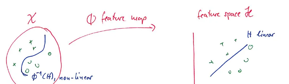
With data in ${\mathbb{R}}^d$ we could fit a linear model $f(x)=w^{\top }x$, $\hat{w}={\mathrm{argmin}}_w\Vert Xw-y{\Vert }^2$. But linear relationships are often not powerful enough. Keep the simplicity of linear methods and still get non-linear: map the inputs to a feature space first and apply OLS there:

$$x_i⟼\phi (x_i)\in {\mathbb{R}}^D,\hat{f}(x_i)={\hat{w}}^{\top }\phi (x_i)$$

If $\phi$ is non-linear, the model is non-linear in $x$ but linear in $\phi (x)$, so OLS still works.

Slide 44: a linear classifier in the feature space corresponds to a non-linear one in the input space.

Examples of basis functions

• Polynomial basis (data in $\mathbb{R}$): $\phi (x)=(1,x,x^2,\dots ,x^p)$. In ${\mathbb{R}}^d$ use products of powers of coordinates such as $(x^{(2)}{)}^3(x^{(5)}{)}^3$; with all combinations the number of features grows as $O(d^p)$.
• Fourier basis: $\phi (x)=(1,\cos (x),\sin (x),\cos (2x),\sin (2x),\dots )$. Natural for periodic signals; any square-integrable function can be approximated arbitrarily well with enough terms.
• Radial basis functions (RBF): centers $c_1,\dots ,c_D\in {\mathbb{R}}^d$ and a scale $\sigma$, ${\phi }_j(x)=\exp (-\frac{\Vert x-c_j{\Vert }^2}{2{\sigma }^2})$: each basis function is a Gaussian centered at $c_j$.

The problem with explicit basis construction: it is not clear how to choose the basis and set its parameters. Much of machine learning since around 2000 tries to avoid constructing a basis explicitly.

Kernel methods: implicit feature maps

Slides 48-53

(Literature: chapters in Understanding Machine Learning, Hastie and Tibshirani, Bach, …; whole books by Schölkopf and Smola (algorithms and some theory) and Steinwart (pure theory).)

The idea of kernel methods is a non-linear feature mapping $\phi$ without ever computing it explicitly. This works whenever a linear algorithm can be expressed purely in terms of scalar products $⟨x_i,x_j⟩$ of the input points.

Kernel trick

Given points in some space $\mathcal{X}$, we would like to embed them (implicitly) into a space via a non-linear feature map $\Phi$ and use a linear method there. Instead of computing the embedding, we use a kernel function

$$k(x,y)=⟨\Phi (x),\Phi (y)⟩$$

This is the kernel trick, and the algorithms are kernel methods.

Slide 52: the kernel computes the scalar product in the feature space directly from the data points.

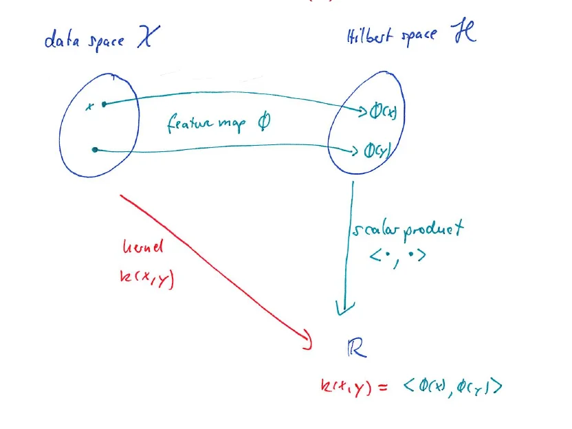
A big part of ML research between 2000 and 2010 went into kernel methods. The most prominent algorithm is the support vector machine: essentially a linear classifier with a large margin, but in the feature space. The theory is beautiful but not part of this lecture.

Memory aid

A kernel is a scalar product in feature space, computed without going there.

Task: feature map and kernel

Exam-style task: a polynomial kernel (4 P)

Math: scalar product

For $x=(x_1,x_2)\in {\mathbb{R}}^2$ consider the kernel $k(x,y)=(x^{\top }y{)}^2$.

(a) (1 P, easy) Compute $k(x,y)$ for $x=(1,2)$ and $y=(3,-1)$.

(b) (1.5 P, harder) Find a feature map $\Phi :{\mathbb{R}}^2\to {\mathbb{R}}^3$ with $k(x,y)=⟨\Phi (x),\Phi (y)⟩$, and check it on the numbers of (a).

(c) (1.5 P, transfer) A linear classifier in the feature space, $\mathrm{sign}(⟨w,\Phi (x)⟩+b)$, can produce which decision boundaries in ${\mathbb{R}}^2$? Why is the kernel useful when $x\in {\mathbb{R}}^{1000}$ and the degree is 3?

Solution

(a) $x^{\top }y=3-2=1$, so $k(x,y)=1$. (1 P)

(b) $(x_1{y}_1+x_2{y}_2{)}^2=x_1^2{y}_1^2+2x_1{x}_2{y}_1{y}_2+x_2^2{y}_2^2$, so $\Phi (x)=(x_1^2,\sqrt{2}{x}_1{x}_2,x_2^2)$. Check: $\Phi (x)=(1,2\sqrt{2},4)$, $\Phi (y)=(9,-3\sqrt{2},1)$, $⟨\Phi (x),\Phi (y)⟩=9-12+4=1$ ✓. (1.5 P)

(c) $w_1{x}_1^2+\sqrt{2}{w}_2{x}_1{x}_2+w_3{x}_2^2+b=0$: conic sections centered at the origin (ellipses, hyperbolas, pairs of lines), i.e. non-linear boundaries in ${\mathbb{R}}^2$. For $x\in {\mathbb{R}}^{1000}$ and degree 3 the explicit map has of the order $1000^3/6\approx 1.7\cdot 10^8$ coordinates, while $k(x,y)=(x^{\top }y{)}^3$ costs one scalar product of length 1000: the kernel trick avoids computing $\Phi$. (1.5 P)

Implicit features vs. representation learning

Slide 54

When kernels were “invented”, people had already realized that good representations are hard to design by hand. The conclusion then: avoid explicit representations altogether and use kernel functions. Nowadays we have (in some applications!) enough data and compute to learn good representations from scratch. Deep networks do this: the last layer is an explicit representation of the data in a very high-dimensional space, learned by the network; on top of it we typically apply a linear method.

Random feature models

Slides 55-67

(Literature: Rahimi and Recht, “Random features for large-scale kernel machines”, NeurIPS 2007; briefly in Hardt and Recht Sec. 4; Bach Sec. 7.4.3, which needs kernels first.)

Random Fourier features. A square-integrable $f\in L^2({\mathbb{R}}^d)$ has a representation $f(x)={\int }_{{\mathbb{R}}^d}c(\omega )\cos ({\omega }^{\top }x+b(\omega ))d\omega$ with frequencies $\omega$, amplitudes $c(\omega )$ and phases $b(\omega )$. Instead of the integral we could use a finite sum over selected frequencies, but we do not know which frequencies matter. Funny idea: sample the frequencies randomly.

Random Fourier features

Step 1: a new, random representation. Draw independently

$${\omega }_1,\dots ,{\omega }_D\stackrel{iid}{\sim }\mathcal{N}(0,{\sigma }^{-2}{I}_d),b_1,\dots ,b_D\stackrel{iid}{\sim }\mathrm{Uniform}[0,2\pi ]$$

The $j$-th random feature of $x\in {\mathbb{R}}^d$ is $Z_j=\cos ({\omega }_j^{\top }x+b_j)$, so $x\mapsto (Z_1,\dots ,Z_D)\in {\mathbb{R}}^D$ (typically $D$ large).

Step 2: learn a linear model on it. With the random features fixed, learn

$$f(x)=\sum _{j=1}^D{a}_j\cos ({\omega }_j^{\top }x+b_j)$$

by least squares (or related methods) for the parameters $a_j$.

The sampling distribution of the ${\omega }_j$ determines which functions are approximated well (Gaussian weights for smooth functions, heavy-tailed distributions give less smooth functions).

Slide 59: a random feature model is a one-hidden-layer network with D neurons, random fixed weights wᵢⱼ and offsets bⱼ, cosine activation, and trained output weights aⱼ.

Random ReLU features and general random features

• ReLU: $f(x)={\sum }_{j=1}^m{a}_j(w_j^{\top }x+b_j{)}_{+}$ with $\sigma (x)=\max \{0,x\}$; $w_j$, $b_j$ are initialized randomly and kept fixed, only the $a_j$ are trained.
• General: a parametric family of basis functions $\mathcal{B}=\{b_{\theta }\mid \theta \in \Theta \}$; draw ${\theta }_1,\dots ,{\theta }_D$ from a distribution $\mu$ on $\Theta$ and use $\phi (x)=(b_{{\theta }_1}(x),\dots ,b_{{\theta }_D}(x){)}^{\top }$ and $f(x)={\sum }_j{a}_j{b}_{{\theta }_j}(x)$. The basis functions should be linearly independent, ideally nearly orthogonal.

From random features to kernels

The empirical kernel of a random feature map and its expectation:

$$\begin{array}{rl}{k}_{emp}(x,x^{\prime })& =\frac{1}{D}\sum _{j=1}^D{b}_{{\theta }_j}(x)b_{{\theta }_j}(x^{\prime })\\ k_{expected}(x,x^{\prime })& =E_{\theta }(b_{\theta }(x)b_{\theta }(x^{\prime }))=\int b_{\theta }(x)b_{\theta }(x^{\prime })d\mu (\theta )\end{array}$$

Under suitable assumptions this is a kernel (a similarity between points). For random Fourier features, $⟨\phi (x),\phi (x^{\prime })⟩\approx k_{Gauss}(x,x^{\prime })$, the better the larger $D$ (Rahimi and Recht). Random ReLU features give the ReLU kernel (neural network Gaussian process kernel, Bach book): the ReLU random feature network approximates a kernel classifier.

The other way round: under some conditions a kernel has a representation $k(x,x^{\prime })={\int }_{\Theta }\phi (x,\theta )\phi (x^{\prime },\theta )d\mu (\theta )$ (Bochner’s theorem for shift-invariant kernels; Mercer), and sampling ${\theta }_1,\dots ,{\theta }_D$ from $\mu$ gives $\hat{k}(x,x^{\prime })={\sum }_j\phi (x,{\theta }_j)\phi (x^{\prime },{\theta }_j)$. In practice deriving $\mu$ and $\phi$ for a given kernel is difficult.

Trap

Slide 66 writes the approximation without the factor $\frac{1}{D}$; as a Monte Carlo estimate of the integral it needs the average $\frac{1}{D}{\sum }_j$ (or features scaled by $1/\sqrt{D}$).

Why random features matter

They connect neural networks and kernel methods in an elegant way, and they are a simple model to study properties of neural networks: the double descent curve of Lecture 8 is shown with random features.

Representation learning

Slides 68-71

So far the representation was fixed in advance (hand-designed $\Phi$, implicit via kernels, random features). Representation learning learns it from data: start from raw data (pixels, tokens, a time series) and train a neural network; each layer of the trained network is a representation, $x\mapsto h_1(x)\mapsto \cdots \mapsto h_L(x)$, and the last layer is the learned representation used for the final prediction.

	Hand-designed features	Learned features
needs	domain knowledge (use it if you have it)	a huge amount of data
risk	might miss important aspects	hard or impossible to interpret; difficult to sanity-check and debug
good for	problems we understand	images and text, where we do not know good features

Validation and benchmarking

Benchmarking in machine learning

Slides 72-77

(Literature: Hardt, The Emerging Science of Machine Learning Benchmarks (parts of the material and many figures); Liao, Taori, Raji and Schmidt, “Are we learning yet? A meta review of evaluation failures across machine learning”, NeurIPS Datasets and Benchmarks 2021; König, Pawelczyk, von Luxburg and Bordt, “Validity Threats for Foundation Model Research”, arXiv 2026.)

For a long time, researchers compared their algorithms on the same benchmarks over and over (ImageNet top-1 accuracy from AlexNet 2012 to ConvNeXt and ViTs 2022). This raises many questions: does the community overfit on particular benchmarks? How to construct benchmarks that report something worthwhile? Do results carry over to the real world? What if the benchmark is only a rough proxy? Which tasks can be evaluated on benchmarks at all? By now benchmark scores have become a strategic target for big companies, which raises more questions: how to measure performance fairly, which benchmarks to use and who decides, how to combine many benchmarks into a ranking (impossibility results in voting and ranking), and how to set incentives against strategic behavior.

Four notions of validity

Slides 78-80

Already in the 1960s the social sciences asked similar questions and developed a framework of validity types.

Four notions of validity

Validity	General question	Illustrated on ImageNet
statistical	Is an estimate on a finite sample representative of the underlying distribution?	Are performance differences statistically reliable, or due to randomness? Is 0.2% better “true” or sampling?
internal	Does the study identify a causal effect within the studied sample, free of confounding and bias?	Are differences caused by the models, not by artifacts of the data set, pre-processing or evaluation protocol?
external	Do the findings generalize to other populations or setups?	Do results generalize to other data sets, tasks or real-world settings?
construct	Does the study capture the intended abstract concept?	Does “ImageNet accuracy” measure “object recognition”?

Keeping them apart

• Statistical = chance (sample size, variance, significance).
• Internal = cause within the study (confounders, artifacts, protocol).
• External = transfer to other settings.
• Construct = what is measured vs. what we mean (the measurement problem of the first part of this lecture).

Memory aid

Four questions: Chance? Cause? Carry over? Concept? Statistical, internal, external, construct.

Practice: which validity is threatened?

Twelve scenarios written for these notes. Pick the validity that is threatened most directly; the explanation points to the slide.

Internal and external validity of ML benchmarks

Slides 81-89

Suppose the community focuses on one benchmark, runs many architectures and ranks them by test score. How meaningful are these scores?

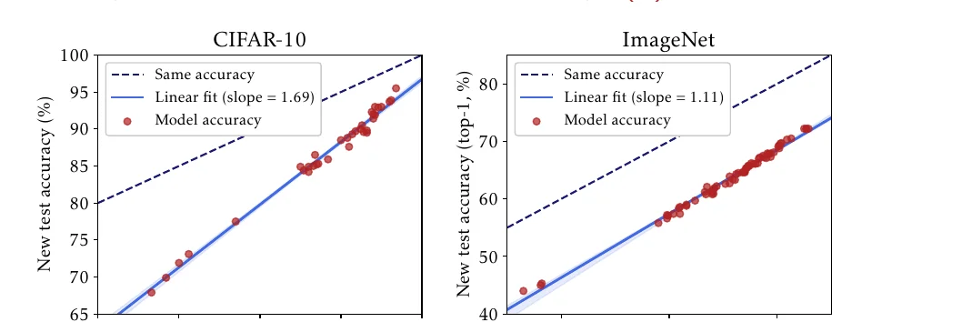
To find out whether the community overfits on benchmarks, researchers carefully recreated test sets for widely used benchmarks, following the original procedure (Recht, Roelofs, Schmidt and Shankar, “Do ImageNet classifiers generalize to ImageNet?”, ICML 2019; Yadav and Bottou, “Cold Case: The Lost MNIST Digits”, NeurIPS 2019). Two findings:

• Accuracy numbers drop significantly between the old and the new test set (expected; limited internal validity of the scores themselves).
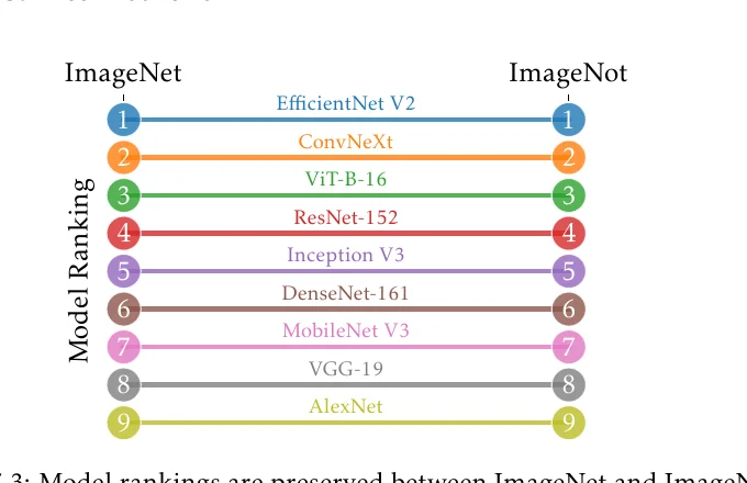
• Model rankings are largely preserved (surprising; internal validity holds for rankings).

Slide 84 (from Hardt's benchmark book): original vs. new test accuracy for CIFAR-10 and ImageNet, one point per model. All points lie below the diagonal, but on a line: the ordering is kept.

External validity beyond ImageNet? Do rankings carry over to other benchmarks? Re-evaluations on many vision data sets (Kornblith, Shlens and Le, “Do better ImageNet models transfer better?”, CVPR 2019; Salaudeen and Hardt, “ImageNot: A contrast with ImageNet preserves model rankings”, arXiv 2024) found: surprisingly, rankings still carried over, and even the relative improvements from one architecture to the next are about the same on ImageNet and ImageNot.

Slide 87: model rankings are preserved between ImageNet and ImageNot.

Summary: scores vs. rankings

• Absolute benchmark numbers satisfy code re-execution and replication under i.i.d. sampling, but little more: even benign distribution shifts change them significantly. They have no external validity.
• Relative comparisons and rankings robustly satisfy internal validity; they replicate under reasonable recreations of the testing conditions and are sometimes stable under major data set variation (signs of external validity).
• The scope of external validity is not fully known.

Validity threats in foundation model research

Slides 90-100

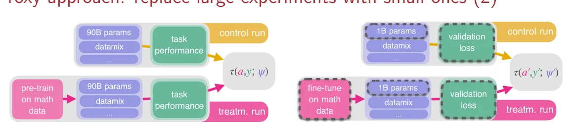
(König, Pawelczyk, von Luxburg and Bordt, “Validity Threats for Foundation Model Research”, arXiv 2026.) Foundation model and LLM research asks big questions whose answers would require training many foundation models in different setups. With limited compute (in particular in academia), researchers run proxy experiments. The savings come at the cost of hidden and sometimes untestable assumptions, which introduce validity threats.

Approach	What it does	Key validity threats
proxy approach	replace large experiments by small ones: a small proxy model instead of a large one, fine-tuning instead of pre-training, validation loss instead of task performance	external validity: do the results still hold in the target setting? (plus construct validity of proxy outcomes)
observational approach	instead of running experiments, analyze public meta-data of existing models (leaderboards, model platforms, technical reports) and relate training choices to outcomes	internal validity (causal claims from observational data); statistical validity (enough independent data?)
single-run approach	one large run contains many independently treatable units (for example documents inserted a number of times to measure memorization): many small experiments in parallel	internal validity (are the units really independent and exchangeable?); external validity

Slide 93: the proxy approach replaces the model, the treatment and the outcome by cheaper proxies.

Summary

Machine learning is so complex that trial-and-error and a naive train/test setup do not give firm conclusions. We need scientific approaches to validation (they largely do not exist yet) and should discuss validity threats of our own setups, ideally in every published paper.

Summary

Topic	Key message
measurement	ML learns the measurement, not the construct; proxies can create bias
data harms	under-representation, sampling bias, historical bias, privacy, copyright; more data does not fix bias
good practice	question the measurement, check representativeness, datasheets
features	explicit feature maps and basis functions; kernels $k=⟨\Phi ,\Phi ⟩$; random features (fixed random first layer, train $a_j$); learned representations
validity	statistical (chance), internal (cause), external (transfer), construct (what is measured)
benchmarks	scores do not replicate under recreated test sets, rankings do
foundation models	proxy (external), observational (internal, statistical), single run (internal, external)

Self-Test

Question cards (12)

What is the difference between a target construct and a measurement procedure? Give two examples.

Answer

The construct is the abstract, often unobservable concept (intelligence, kidney function); the measurement is the device that produces numbers (IQ test score, creatinine level). The measurement can be a poor approximation of the construct.

Why did the US health insurance algorithm show racial bias?

Answer

It predicted health care costs as a proxy for illness. Because less money is spent on Black patients with the same illness (unequal access), Black patients were considerably sicker at the same risk score.

Why did the UK liver matching system disadvantage young patients?

Answer

Instead of life-years gained it predicted the probability of surviving 5 years with and without transplant (data availability). Young patients are likely to survive 5 years anyway, so their predicted benefit was small and older patients were preferred.

What does "categories become normative" mean?

Answer

How we measure a concept changes how we think about it: widely used classification systems (census categories, binary sex categories) shape societal norms.

Name four harms that can come with data.

Answer

Under-represented minorities, sampling bias (crime data reflects police activity), historical biases and stereotypes, offensive or illegal content, privacy violations (anonymization is not enough, Netflix), copyright violations.

Why can more data not fix a biased data set?

Answer

More data averages out unbiased noise, but a systematic bias stays: the model converges to the biased quantity. The model cannot fix data problems in hindsight.

What are datasheets for datasets?

Answer

Documentation accompanying every data set (Gebru et al. 2018): motivation, composition, collection process, pre-processing decisions, recommended uses, known limitations; for transparency, accountability and reproducibility.

How do basis functions make linear methods non-linear? Give three examples.

Answer

Map $x\mapsto \phi (x)$ and fit a linear model $w^{\top }\phi (x)$: non-linear in $x$, linear in $\phi (x)$, so OLS still applies. Polynomial $(1,x,\dots ,x^p)$, Fourier $(1,\cos x,\sin x,\dots )$, RBF $\exp (-\Vert x-c_j{\Vert }^2/(2{\sigma }^2))$.

What is the kernel trick, and when can it be used?

Answer

Compute $k(x,y)=⟨\Phi (x),\Phi (y)⟩$ directly instead of the feature map; possible whenever the linear algorithm only uses scalar products $⟨x_i,x_j⟩$ of the data points.

Describe random Fourier features. What is learned and what is fixed?

Answer

Draw ${\omega }_j\sim \mathcal{N}(0,{\sigma }^{-2}I)$ and $b_j\sim U[0,2\pi ]$, features $\cos ({\omega }_j^{\top }x+b_j)$, $j=\mathrm{1..}D$; they stay fixed. Only the output weights $a_j$ of $f(x)={\sum }_j{a}_j\cos ({\omega }_j^{\top }x+b_j)$ are learned (least squares). The inner product of the features approximates the Gaussian kernel.

Define the four notions of validity.

Answer

Statistical: is the finite-sample estimate representative (not chance)? Internal: is the effect caused by what we claim, free of confounding? External: do findings generalize to other settings? Construct: does the measurement capture the intended concept?

What did recreated test sets for CIFAR-10 and ImageNet show?

Answer

All models lost accuracy significantly (absolute scores lack validity), but the rankings were largely preserved (internal validity of rankings); rankings even carried over to ImageNot (some external validity).

Multiple Choice

Multiple choice (8)

A study reports that model A beats model B by 0.1% accuracy on a small test set, without error bars. Which validity is most directly in question?

• statistical validity

• internal validity

• external validity

• construct validity

Explanation

Whether such a small difference is more than sampling randomness is the question of statistical validity (slide 80).

"Does ImageNet accuracy actually measure object recognition?" asks about

• statistical validity

• internal validity

• external validity

• construct validity

Explanation

It is about whether the metric (measurement) captures the intended concept (construct).

The key validity threat of the proxy approach (small model instead of a large one) is

• statistical validity

• internal validity

• external validity

• none, the proxy approach is valid by construction

Explanation

Slide 93: do the results still hold in the target setting? The observational approach mainly threatens internal validity.

What did the recreated ImageNet and CIFAR-10 test sets show?

• Accuracy stayed the same, but rankings changed.

• Accuracy dropped significantly, but rankings were largely preserved.

• Both accuracy and rankings stayed the same.

• Both accuracy and rankings changed completely.

Explanation

Scores lack validity, rankings have internal (and some external) validity (slides 83-89).

In a random Fourier feature model, which parameters are trained?

• the frequencies ${\omega }_j$ and the offsets $b_j$

• only the output weights $a_j$

• all weights, by backpropagation

• none, the model is a kernel

Explanation

The first layer is drawn at random and kept fixed; step 2 fits $a_j$ by least squares.

What does the kernel trick avoid?

• computing scalar products

• computing the (possibly very high-dimensional) feature map explicitly

• choosing a loss function

• the need for training data

Explanation

$k(x,y)=⟨\Phi (x),\Phi (y)⟩$ is evaluated directly; the algorithm only needs scalar products.

A hospital predicts future health care costs to allocate care to the sickest patients. The main problem is

• too few training points

• a mismatch between the target construct (illness) and the measurement (costs)

• overfitting of the model

• a non-convex loss

Explanation

Obermeyer et al.: the model learns the measurement; unequal spending turns the proxy into a source of racial bias.

Which statement about anonymized data sets is true?

• Removing names guarantees privacy.

• Anonymized data sets can often be de-anonymized by linking them to public data.

• Public availability on the internet grants the right to use data for training.

• More data removes privacy risks.

Explanation

Netflix ratings were de-anonymized by comparing them to public ratings (Narayanan and Shmatikov 2008). Public availability does not imply permission (copyright).

Cheat sheet and full integration tasks

This lecture is mostly about terms, so the first task is one scenario in which every term has to be applied once. The second task covers the two calculations of the lecture, a kernel with its feature map and a random feature model. Write your own sheet first, solve the tasks with it next to you, then open the sheet at the bottom and compare. The letters in brackets name the block of the sheet that a subtask needs.

Full integration task: one study, every term (12 P)

A company trains a model that ranks job applicants by predicted “job performance”. The label is the rating that a manager gave after the first year. The training data are 2000 past hires at the two main sites. On a test set of 500 employees model A reaches 81.2% accuracy and model B 80.9%. A was trained with a newer preprocessing pipeline than B.

(a) (2 P, block A) Name the target construct and the measurement procedure. What does the model learn, and why is that risky here?

(b) (2 P, block A) Name two problems of this data set that more data of the same kind would not fix.

(c) (4 P, block B) Four people doubt the claim “A is better than B”. Which kind of validity does each doubt concern?

1. “0.3 points on 500 test employees can be chance.”
2. “A and B were preprocessed differently, so the gain may not come from the model.”
3. “Will A still be better at the new site in another country?”
4. “Does a manager’s rating reflect performance at all?”

(d) (2 P, block B) A year later the test set is recreated with the same procedure. What do you expect for the two accuracy numbers, and what for the order of A and B?

(e) (2 P, block B) For the next model generation the team cannot afford to retrain the large model. It tests an idea on a small model instead, and it also compares the entries of a public leaderboard to see which training choices help. Which validity threats does each approach bring?

Solution

(a) Target construct: job performance, which is not directly observable. Measurement: the manager’s rating after one year. The model learns the measurement, not the construct. If ratings are systematically lower for some group, the model reproduces exactly that, however accurate it is on the ratings. (2 P)

(b) Sampling bias: the data only contains people who were hired, there are no labels for rejected applicants, and only two sites are covered. Historical bias: past hiring and rating decisions are used as ground truth. Both are systematic, so more data converges to the same wrong quantity. More data only helps against random noise. (2 P)

(c) 1: statistical validity (chance). With $n=500$ the standard error of an accuracy around 0.81 is $\sqrt{0.81\cdot 0.19/500}\approx 0.018$, six times the difference. 2: internal validity (cause): the comparison is confounded by the pipeline. 3: external validity (carry over to another setting). 4: construct validity (does the number measure the concept). (1 P each)

(d) The accuracy numbers drop noticeably: absolute scores do not carry over even to a careful recreation. The order of the two models is likely to stay: rankings replicated in the studies on recreated test sets. Here the two models are so close that even this is uncertain. (2 P)

(e) Small model instead of the large one: the proxy approach. Main threat: external validity, since the result may not hold for the large model, plus construct validity if a proxy outcome such as validation loss replaces the real task. Leaderboard comparison: the observational approach. Threats: internal validity, because causal claims are drawn from observational data, and statistical validity, because there are few independent entries. (2 P)

Full integration task: kernel and random features (8 P)

Math: scalar product · counting

For $x=(x_1,x_2)\in {\mathbb{R}}^2$ consider the kernel $k(x,y)=(1+x^{\top }y{)}^2$.

(a) (2 P, block C) Compute $k(x,y)$ for $x=(1,2)$ and $y=(1,1)$.

(b) (3 P, block C) Find a feature map $\Phi$ with $k(x,y)=⟨\Phi (x),\Phi (y)⟩$ and check it on the numbers of (a).

(c) (1 P, block C) How many coordinates does the explicit feature map have for $x\in {\mathbb{R}}^{100}$, and what does the kernel cost instead?

(d) (2 P, block D) A random Fourier feature model on inputs in ${\mathbb{R}}^{10}$ uses $D=500$ features. Which parameters are random and fixed, which are trained, and how many of each are there? What happens as $D$ grows?

Solution

(a) $x^{\top }y=1+2=3$, so $k(x,y)=4^2=16$. (2 P)

(b) Expand: $(1+x_1{y}_1+x_2{y}_2{)}^2=1+2x_1{y}_1+2x_2{y}_2+x_1^2{y}_1^2+2x_1{x}_2{y}_1{y}_2+x_2^2{y}_2^2$. Every term is a product of an $x$ part and a $y$ part, so

$$\Phi (x)=(1,\sqrt{2}{x}_1,\sqrt{2}{x}_2,x_1^2,\sqrt{2}{x}_1{x}_2,x_2^2)$$

Check: $\Phi (x)=(1,\sqrt{2},2\sqrt{2},1,2\sqrt{2},4)$ and $\Phi (y)=(1,\sqrt{2},\sqrt{2},1,\sqrt{2},1)$, with scalar product $1+2+4+1+4+4=16$. (3 P)

(c) All monomials of degree at most 2 in 100 variables: $1+100+100+\left(\genfrac{}{}{0ex}{}{100}{2}\right)=5151$ coordinates. The kernel needs one scalar product of length 100 and one square. (1 P)

(d) Random and fixed: the frequencies ${\omega }_j\in {\mathbb{R}}^{10}$ and the phases $b_j$, together $500\cdot 10+500=5500$ numbers. Trained: only the 500 output weights $a_j$, by least squares, because the model is linear in the features. As $D$ grows, the scalar product of the feature vectors (with the factor $\frac{1}{D}$) approaches the Gaussian kernel. (2 P)

Cheat sheet: data, features and validity (5 blocks)

A. Construct, measurement and data problems

You see	It means
the label is a stand-in (cost for illness, rating for performance)	proxy target: the model learns the measurement, not the construct
the plan is to collect more data	helps against random noise, not against a systematic bias
a group is rare in the data	under-representation: poor performance on that group
the data exists only where someone looked (recorded crime, hired applicants)	sampling bias
past decisions used as labels	historical bias is learned as ground truth
names removed from the data	not anonymous: records can be re-identified
a data set without documentation	missing datasheet: motivation, collection, limits unknown

B. The four validities

Validity	Key word	The doubt sounds like
statistical	chance	too few test points, not significant, could be random
internal	cause	a confounder, an artifact, a different protocol or pipeline explains the difference
external	carry over	another data set, another site, a larger model, the real world
construct	concept	does this number measure what we mean?

Ask in this order: Is it about randomness? About the cause inside the study? About another setting? About the meaning of the measurement?

You see	It means
benchmark scores on a recreated test set	the numbers drop: absolute scores have no external validity
model rankings on a recreated or different test set	largely preserved: rankings have internal validity and signs of external validity
a small proxy model or a proxy metric	threat to external validity, and to construct validity for the proxy outcome
conclusions from leaderboards and model cards	observational: threats to internal and statistical validity
many units inside one large run	threats to internal validity (are the units independent?) and external validity

C. Kernel and feature map by hand

1. A kernel is a scalar product in feature space: $k(x,y)=⟨\Phi (x),\Phi (y)⟩$.
2. To find $\Phi$: expand $k(x,y)$, write every term as (something in $x$) times (the same thing in $y$), and split numerical factors evenly with a root.
3. Check with numbers: compute $k(x,y)$ directly and through $\Phi$.

Kernel on ${\mathbb{R}}^2$	Feature map
$(x^{\top }y{)}^2$	$(x_1^2,\sqrt{2}{x}_1{x}_2,x_2^2)$
$(1+x^{\top }y{)}^2$	$(1,\sqrt{2}{x}_1,\sqrt{2}{x}_2,x_1^2,\sqrt{2}{x}_1{x}_2,x_2^2)$

• A linear classifier in feature space is a non-linear boundary in the input space (for degree 2: ellipses, hyperbolas, pairs of lines).
• The explicit map of degree $p$ in $d$ dimensions has of the order $d^p$ coordinates. The kernel costs one scalar product.

D. Random features

Part	Random Fourier features
drawn once and frozen	${\omega }_j\sim \mathcal{N}(0,{\sigma }^{-2}{I}_d)$ and $b_j\sim \mathrm{Uniform}[0,2\pi ]$: $Dd+D$ numbers
feature	$Z_j=\cos ({\omega }_j^{\top }x+b_j)$
trained	the $D$ weights $a_j$ of $f(x)={\sum }_j{a}_j{Z}_j$, by least squares
as a network	one hidden layer with a random, frozen first layer and a trained output layer
kernel	$\frac{1}{D}{\sum }_j{Z}_j(x)Z_j(x^{\prime })$ approaches the Gaussian kernel as $D$ grows. ReLU features give the ReLU kernel

E. Traps

• Internal is about the cause inside the study, external about other settings. A different preprocessing is internal, a different country is external.
• A high accuracy on a proxy label says nothing about construct validity.
• Scores and rankings behave differently: scores do not transfer, rankings mostly do.
• The feature map of $(x^{\top }y{)}^2$ needs the factor $\sqrt{2}$ on the mixed term.
• In a random feature model the first layer is not trained.

References

All sources cited on the slides, in slide order (20 entries)

Slide	Source	Key point
6, 55	Hardt and Recht, Patterns, Predictions, and Actions, Sec. 4 (online)	measurement; random features
12	Obermeyer, Powers, Vogeli and Mullainathan, “Dissecting racial bias in an algorithm used to manage the health of populations”, Science, 2019	cost as a proxy for illness
14	AI Snake Oil, “Does the UK’s liver transplant matching algorithm systematically exclude younger patients?“	5-year survival as target
24	Narayanan and Shmatikov, “Robust de-anonymization of large sparse datasets”, 2008	Netflix de-anonymization
24	Dwork et al., “Exposed! A survey of attacks on private data”, 2017	privacy attacks
31	Gebru et al., “Datasheets for datasets”, 2018	documentation of data sets
48	Understanding Machine Learning; Hastie and Tibshirani; Bach	kernels in textbooks
48	Schölkopf and Smola; Steinwart	books on kernel methods
55, 64	Rahimi and Recht, “Random features for large-scale kernel machines”, NeurIPS 2007	random Fourier features
55, 64	Bach, Learning Theory from First Principles, Sec. 7.4.3	random features, ReLU kernel
72	Hardt, The Emerging Science of Machine Learning Benchmarks	benchmarks, figures
72	Liao, Taori, Raji and Schmidt, “Are we learning yet? A meta review of evaluation failures across machine learning”, NeurIPS Datasets and Benchmarks 2021	evaluation failures
72, 90	König, Pawelczyk, von Luxburg and Bordt, “Validity Threats for Foundation Model Research”, arXiv 2026	validity threats
76	Epoch AI (image, April 2026)	benchmark scores as strategic targets
83	Recht, Roelofs, Schmidt and Shankar, “Do ImageNet classifiers generalize to ImageNet?”, ICML 2019	recreated test sets
83	Yadav and Bottou, “Cold Case: The Lost MNIST Digits”, NeurIPS 2019	recreated MNIST test set
86	Kornblith, Shlens and Le, “Do better ImageNet models transfer better?”, CVPR 2019	transfer of rankings
86	Salaudeen and Hardt, “ImageNot: A contrast with ImageNet preserves model rankings”, arXiv 2024	rankings preserved
65	Bochner’s theorem; Mercer’s theorem	kernels as integrals over features
25	New York Times v. OpenAI (ongoing lawsuit)	copyright of training data

Related

• Previous: Lecture 6: Aggregation, Bagging and Boosting · Next: Lecture 8: Overparameterized Learning · Course: Overview · Formula Sheet · Glossary
• Concepts: Measurement and Construct, Kernel Methods, Random Features, Validity, Inductive Bias
• Exercises: Sheet 7, Exercises 1-2 (weighted linear regression, interpreting coefficients)