Lecture 8: Overparameterized Learning

TL;DR

1. Puzzle: deep networks have far more parameters than data points, are trained to training error 0 (they can even fit random labels), and still generalize. Classical bounds (VC, Rademacher) are vacuous here.
2. Double descent: the test error rises towards the interpolation threshold (as many parameters as data points) and can fall again beyond it, sometimes below the classical optimum. It does not always happen (polynomial regression), and its shape depends on how parameters are counted.
3. Implicit regularization: GD on over-parameterized least squares started at $w_0=0$ converges to the minimum norm solution $w^{\star }=X^{\top }(X{X}^{\top }{)}^{-1}y$ (Theorem 1: GD finds the minimum norm solution). GD on the logistic loss for separable data converges in direction to the max-margin separator (Theorem 2: max-margin bias of GD). The optimizer picks one special solution among many.
4. Benign overfitting: the minimum norm interpolator can fit pure noise and still predict well. Toy setup (true function 0): risk ${\sigma }^{2}n/(d-n-1)\to 0$ for $d\gg n$ (Theorem 3: benign overfitting in the toy setup). Geometry: spiky-smooth, narrow spikes at the training points with vanishing volume, smooth elsewhere.
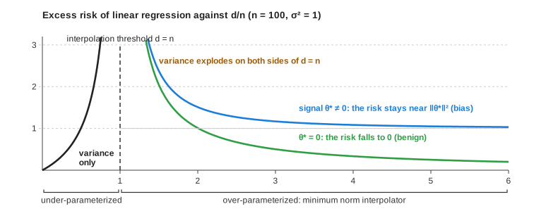
5. Not always benign: isotropic Gaussian inputs with a signal ${\theta }^{\ast }$: variance ${\sigma }^{2}n/(d-n-1)$ is small, but the bias $\Vert {\theta }^{\ast }{\Vert }^2(d-n)/d$ stays (Theorem 4: excess risk in both regimes). Benign overfitting needs an aligned covariance: few large eigenvalues that carry the signal plus a long, flat tail of small eigenvalues that absorbs the noise (Theorem 5: excess risk for a general covariance, four regimes).
6. Why large models: two-layer networks are universal approximators (Theorem 6: universal approximation), but GD can need exponentially many steps to learn a small network (Theorem 7: hardness of learning a small network). Robust interpolation (Lipschitz constant 1) needs $p\gtrsim nd$ parameters (Bubeck and Selke). Over-parameterized loss landscapes have many connected global minima; very wide networks behave like kernel methods (NTK, no feature learning).

Exam relevance

• Real exam, task 1 (multiple choice): a question on over- vs. under-parameterization appeared. Know which effects belong to which regime, where the interpolation threshold is, and what the formulas of Theorem 4 (excess risk in both regimes) say.
• Mock exam: a full task on spiky-smooth interpolation in high dimensions (union bound over the spikes, why the volume vanishes). Practice with the spike task.
• Computations: the minimum norm solution by hand, interpolation thresholds, evaluating the excess risk formulas and reading the variance and bias terms of Theorem 5 (excess risk for a general covariance).
• Sheet 6, Exercise 2 (linear regression in different regimes), Sheet 9, Exercise 1 (the second descent for random features), Sheet 10, Exercise 1 (loss curves and the four regimes of linear regression).
• Everything in one go: the cheat sheet with two full integration tasks at the end of this note.

Exam essentials (7 cards)

Only what you should know by heart in the exam. Click a card for the answer, or press a to go through them as flashcards. For Anki: deck of this lecture.

What is double descent?

Answer

The test error rises towards the interpolation threshold (as many parameters as data points) and can fall again beyond it.
Classical bounds (VC, Rademacher) are vacuous in this regime.

Which solution does GD find for over-parameterized least squares ( $d>n$)?

Answer

Started at $w_0=0$: the minimum norm solution $w^{\star }=X^{\top }(X{X}^{\top }{)}^{-1}y$.
This is implicit regularization: the optimizer picks one solution among many.

Where does GD on the logistic loss converge for separable data?

Answer

In direction to the max-margin separator.

Risk with isotropic inputs: under- vs. over-parameterized?

Answer

Under ($d<n$): $\frac{{\sigma }^{2}d}{n-d-1}$. Over ($d>n$): $\frac{{\sigma }^{2}n}{d-n-1}+\Vert {\theta }^{\ast }{\Vert }^2\frac{d-n}{d}$.
Both blow up at $d\approx n$.

Why is overfitting with isotropic inputs not benign?

Answer

For $d\gg n$ the variance ${\sigma }^{2}n/(d-n-1)$ is small, but the bias $\Vert {\theta }^{\ast }{\Vert }^2(d-n)/d$ stays.

When is overfitting benign?

Answer

With an aligned covariance: a few large eigenvalues carry the signal,
and a long, flat tail of small eigenvalues absorbs the noise.

Spiky-smooth interpolation: why do the spikes not hurt?

Answer

The interpolator has narrow spikes at the training points and is smooth elsewhere.
Union bound over $n$ spikes: $P\le 2n{e}^{-cd{t}^2}$, which vanishes once $d$ grows faster than $\log n$.

Overview: 1. Puzzling empirical results, 2. The double descent curve, 3. Implicit regularization by the optimizer, 4. Benign overfitting (toy setup, isotropic model, aligned covariance, relation to classical theory), 5. Why do we need large models?, 6. The loss landscape, 7. Infinite width and the neural tangent kernel, 8. Take home.

Puzzling empirical results

Learning in the over-parameterized regime

Slides 6-7

In the over-parameterized regime we deal with models that have many more parameters than we have data points. Intuitively, the model could simply memorize the training data without any generalization. Hence it is super-surprising that machine learning works in this regime.

• Images: a neural network with, say, 20 million parameters is trained on ImageNet (1 million images).
• Language: GPT-4 has about $10^{10}$ parameters, its training data of the order of $10^{12}$ tokens. That sounds like more tokens than parameters, but the number of tokens may not be the right way to count: the “effective signal” in this data is believed to be much smaller. Similarly, the number of parameters might not be the best measure of model size.
• Also in much simpler applications, people train deep networks with many parameters on relatively few points, and it often works.

Overfitting might not hurt

Slides 8-9

The first big surprise: the models are typically trained to fit the training data perfectly (training error 0), and training often continues far beyond that point. Still, the models generalize. This is all the more surprising because the large function classes contain many functions with close to 0 training error, and many of them would not generalize (recall the over-parameterized linear models of Lecture 5).

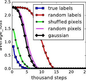
Deep networks can fit random labels (Zhang, Bengio et al., 2017)

Train an MLP on CIFAR-10 (60,000 images, 10 classes) with randomly shuffled labels. The MLP always reaches training error 0. This indicates that the shattering coefficient of the function class is maximal. On ImageNet (1 million images, 1000 random labels) the result looks very similar.

Slide 9: training loss on CIFAR-10. True labels, random labels, shuffled or random pixels: all reach zero training loss, random labels just take longer.

What this means for Lecture 3

If a class can fit any labeling of the training set, its growth function is $2^n$ and the VC and Rademacher bounds of Lecture 3 are vacuous. They are not wrong, they just say nothing about why these networks generalize on real labels.

Local optima and the need for new tools

Slides 10-11

• Why don’t we get stuck in local optima? Deep networks induce highly non-convex optimization problems in very high-dimensional spaces. Yet the optimizers manage to find good local (global?) optima.
• Need new tools: the traditional way of looking at machine learning is not wrong. Its results simply do not shed insight on deep learning, or they must be applied more carefully. We need other tools to explain deep networks.

The double descent curve

The statistics puzzle

Slides 13-14

(Literature: Belkin, Hsu, Ma, Mandal, PNAS 2019; Belkin, “Fit without fear”, Acta Numerica 2021; Bartlett, Montanari, Rakhlin, Acta Numerica 2021.)

In the over-parameterized regime we train to complete overfitting. The traditional bias-variance picture (Lecture 1.2) predicts that the test error explodes. Why is this not the case?

Primer: a random feature example

Slides 15-19

A toy example with few points in a very high-dimensional space, built with a random feature model (Lecture 7):

1. Original data: a low dimension $d=5$ and a low sample size $n=200$. Sample $x_1,\dots ,x_n$ uniformly from the sphere in ${\mathbb{R}}^d$, fix $v^{\ast }\in {\mathbb{R}}^d$ and define the non-linear true function and noisy labels

$$f(x)=(\frac{1}{4}+⟨v^{\ast },x{⟩}^2{)}^{-1},y_i=f(x_i)+{\epsilon }_i,{\epsilon }_i\sim \mathcal{N}(0,{\sigma }^2).$$

2. Transformed data: sample $m$ random vectors $v_1,\dots ,v_m$ from the sphere, map $x$ to $(v_1^{\top }x,\dots ,v_m^{\top }x)$, apply a ReLU and a linear output with parameter vector $\theta$: $f_{\theta }(x)={\sum }_{j=1}^m{\theta }_j(v_j^{\top }x{)}_{+}$. This is a network with $m$ hidden neurons whose first layer is random and fixed.
3. Training: GD on the squared loss, training only the last layer:

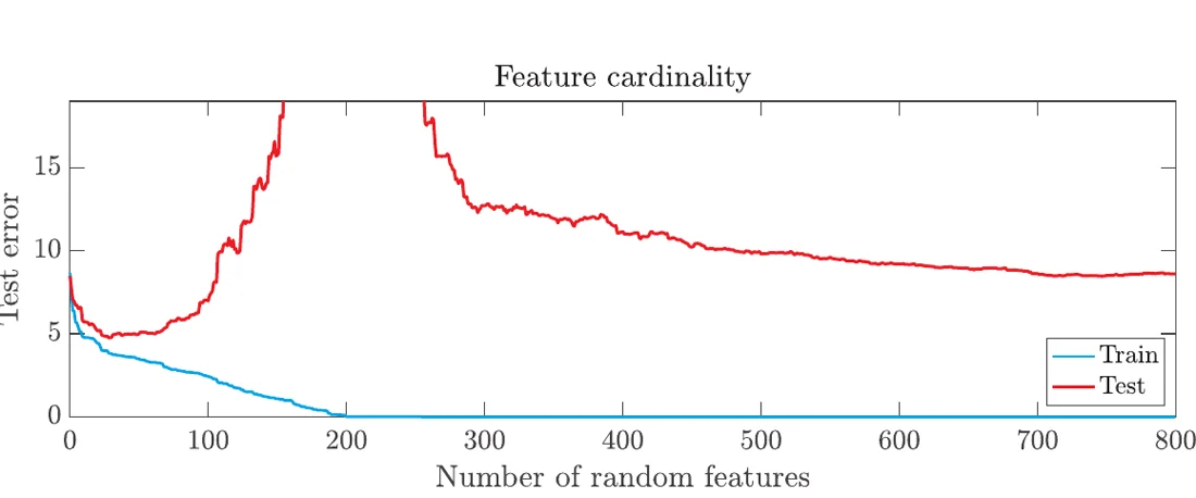
$$\underset{\theta \in {\mathbb{R}}^m}{\min }\sum _{i=1}^n(y_i-\sum _{j=1}^m{\theta }_j(v_j^{\top }{x}_i{)}_{+}{)}^2.$$

Slide 18 (figure from the Bach book): training error (blue) and test error (red) against the number m of random features, n = 200. The test error peaks at m = n and falls again beyond it.

With $m=200=n$ features we have as many parameters as data points: the interpolation threshold. From here on training error 0 is possible. The surprise is the test error: it increases (as expected) as $m$ approaches the threshold from the left, but decreases afterwards. The maths of this example is Sheet 9, Exercise 1. Similar observations hold for many other models.

Double descent in practice

Slides 20-24

Two regimes

• Under-parameterized regime: fewer parameters than data points, cannot interpolate, “traditional” behavior (U-shaped test curve).
• Over-parameterized or interpolation regime: enough parameters to reach training error 0. Here the test risk sometimes decreases dramatically again and sometimes even gets lower than in the traditional regime.

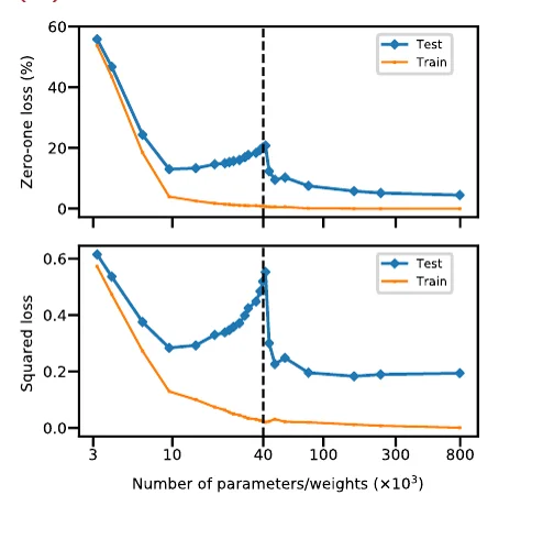
The classical U-curve and the double descent curve of Belkin et al. are shown in Lecture 1.2. In the original paper the behavior was established empirically for a range of algorithms, including neural networks and random forests:

Slide 23: one hidden layer with H units on MNIST (n = 4000, d = 784, K = 10). Threshold at n times K parameters.

Slide 24: random forests on MNIST (n = 10000). Complexity grows first with the leaves per tree, then with the number of trees.

For the network the number of parameters is $(d+1)\cdot H+(H+1)\cdot K$ and the threshold is observed at $n\cdot K$ (one equation per point and class).

Other descent curves

Slides 25-28

The curves do not always show a double descent, many more shapes are possible:

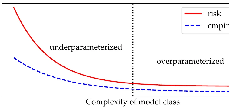
• Single descent: the risk just keeps decreasing with the complexity, with no peak (figure from the Hardt and Recht book).
• Triple (multiple) descent: in models with several random feature layers of different sizes $N_1,N_2$, several peaks can appear (Meng et al., JMLR 2024).
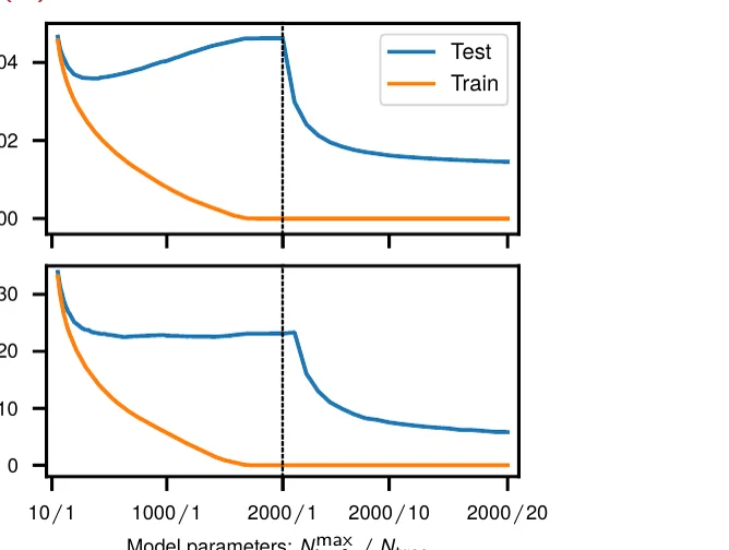
• U-turn: it has been argued repeatedly that the shape strongly depends on how we count the parameters (Curth et al., NeurIPS 2023). For random forests the original paper counts the total number of leaves. But the behavior changes when going from one tree (blue part) to several trees (red part), which introduces the “kink”. Counting leaves per tree $P^{leaf}$ and number of trees $P^{ens}$ separately gives ordinary U-shaped or monotone curves (“back to U”).

Slide 25: single descent. Risk (red) and empirical risk (blue) decrease through both regimes.

A case without double descent

Slides 29-30

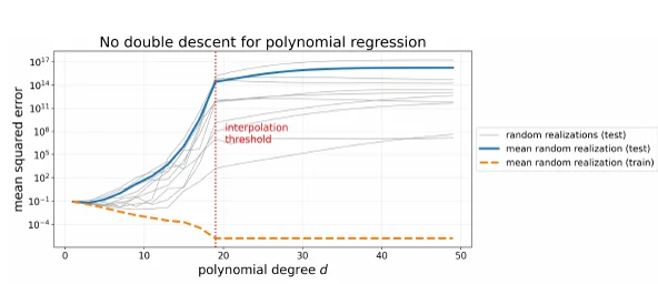
Double descent does not automatically happen. An example where fitting beyond the threshold goes wrong:

• $n=20$ training points $x_i$ uniform in $[-1,1]$ with noisy labels $y_i=\frac{1}{1+25x_i^2}+{\epsilon }_i$.
• Polynomial regression of increasing degree $d$ with the monomial features $1,x,x^2,\dots ,x^d$ and least squares loss ${\min }_{a\in {\mathbb{R}}^{d+1}}\frac{1}{n}{\sum }_{i=1}^n(y_i-{\sum }_{k=0}^d{a}_k{x}_i^k{)}^2$. The interpolation threshold is $d=19$ ($d+1=20$ coefficients).
• Test error on a dense grid in $[-1,1]$: beyond the threshold the high-degree polynomial becomes unstable and the test error grows instead of showing a second descent.

Slide 29: polynomial regression, n = 20. Training error (orange) hits zero at degree 19, the test error (blue, log scale) explodes and never comes down.

Take-home: the curve can go down again

Slides 31-32

Take-home

Learning in the over-parameterized regime can work. The exact shape of the curve is not important. What is important: the curve might (but not always does) show a smaller test error beyond the interpolation threshold.

Empirically, double or multiple descent can happen in many over-parameterized models, and in some models the curves can be derived analytically. To see the intuitive reason we first need two more topics: implicit regularization and benign overfitting. Then we come back to the question.

Task: interpolation thresholds

Exam-style task: where is the interpolation threshold? (4 P)

Math: linear systems

(a) (1 P, easy) A random feature model with $m$ ReLU features is fit by least squares to $n=350$ points. For which $m$ is the interpolation threshold, and what is the training error for $m=500$?

(b) (1.5 P, harder) A network with one hidden layer of $H$ units is trained with squared loss on $n=2000$ images with $d=784$ pixels and $K=10$ classes (one output per class). The number of parameters is $(d+1)H+(H+1)K$. For which $H$ (roughly) do you expect the test error peak?

(c) (1.5 P, transfer) A student fits polynomials of degree $d$ to $n=30$ noisy points with the monomial features and sees the test error rise between $d=20$ and $d=29$. They conclude: “Beyond $d=29$ the test error will come down again, that is double descent.” Assess this.

Solution

(a) At $m=n=350$ the model has as many parameters as equations and can interpolate (the feature matrix has full rank almost surely). For $m=500>n$ the training error is $0$. (1 P)

(b) The threshold is at $n\cdot K=2000\cdot 10=20,000$ parameters. $(785)H+10H+10=795H+10=20,000$ gives $H\approx 25$. Expect the peak around 25 hidden units; below it the classical U-curve, above it possibly a second descent. (1.5 P)

(c) The threshold is at $d=29$ ($d+1=30$ coefficients). But double descent does not happen automatically: for polynomial regression with monomial features the slides show that the test error keeps growing beyond the threshold, because the high-degree interpolating polynomials are unstable (slides 29-30). A second descent needs a benign structure (see below), not just more parameters. (1.5 P)

Implicit regularization by the optimization algorithm

GD converges to the minimum norm solution

Slides 34-36

(Literature: Bach, Learning Theory from First Principles, Sec. 12.1.1.)

Setup: GD for over-parameterized linear least squares

• Over-parameterized: $n<d$. Data $X\in {\mathbb{R}}^{n\times d}$, $y\in {\mathbb{R}}^n$. Assume $X$ has full row rank $n$ (true with probability 1 for Gaussian points). Then $X{X}^{\top }\in {\mathbb{R}}^{n\times n}$ is invertible and perfect interpolation is possible: some $w^{\ast }$ has $X{w}^{\ast }=y$.
• Objective $L(w)=\frac{1}{2}\Vert Xw-y{\Vert }^2$, gradient descent initialized at $w_0=0$:

$$w_{t+1}=w_t-\eta X^{\top }(X{w}_t-y),0<\eta <\frac{2}{{\lambda }_{\max }(X{X}^{\top })}.$$

Theorem 1 (convergence to the minimum norm solution)

In this setup:

1. The GD iterates converge to $w^{\star }=X^{\top }(X{X}^{\top }{)}^{-1}y$.
2. $w^{\star }$ is the minimum norm solution: it solves $Xw=y$, and among all solutions it has the smallest Euclidean norm $\Vert w\Vert$. It is the unique solution with this property.

A similar result holds for SGD.

Proof of Theorem 1

Slides 37-41

Step 1: all iterates lie in $S_n:=\mathrm{span}\{x_1,\dots ,x_n\}=\mathrm{range}(X^{\top })$. Induction: true for $w_0=0$. The update $\eta X^{\top }(X{w}_t-y)$ is a linear combination of training points (for any $v$, $X^{\top }v={\sum }_i{v}_i{x}_i$). So $w_t\in S_n$ implies $w_{t+1}\in S_n$, and we can write $w_t=X^{\top }{\alpha }_t$ for some ${\alpha }_t\in {\mathbb{R}}^n$.

Step 2: the residuals satisfy $r_{t+1}=(I-\eta X{X}^{\top })r_t$. With $r_t:=X{w}_t-y$:

$$r_{t+1}=X(w_t-\eta X^{\top }(X{w}_t-y))-y=(X{w}_t-y)-\eta X{X}^{\top }(X{w}_t-y)=(I-\eta X{X}^{\top })r_t.$$

Step 3: GD is contractive and interpolates in the limit. $X{X}^{\top }$ is symmetric positive semi-definite and $0<\eta <2/{\lambda }_{\max }(X{X}^{\top })$, so all eigenvalues of $I-\eta X{X}^{\top }$ have modulus strictly smaller than 1: a strict contraction. Hence $r_t\to 0$, i.e. $X{w}_t\to y$.

Step 4: the limit is $w^{\star }=X^{\top }(X{X}^{\top }{)}^{-1}y$. $X{w}_t=X{X}^{\top }{\alpha }_t\to y$ and $X{X}^{\top }$ is invertible, so ${\alpha }_t\to (X{X}^{\top }{)}^{-1}y$ and $w_t=X^{\top }{\alpha }_t\to X^{\top }(X{X}^{\top }{)}^{-1}y$.

Step 5: inside $S_n$ there is only one solution. If $w=X^{\top }\alpha \in S_n$ and $Xw=y$, then $X{X}^{\top }\alpha =y$, and since $X{X}^{\top }$ is invertible, $\alpha =(X{X}^{\top }{)}^{-1}y$ is unique.

Step 6: it is the minimum norm solution. Let $w$ be any solution. Decompose orthogonally $w=w_{\parallel }+w_{\perp }$ with $w_{\parallel }\in \mathrm{range}(X^{\top })$ and $w_{\perp }\in \ker (X)$. Then $Xw=X{w}_{\parallel }$, so $w_{\parallel }\in S_n$ is also a solution, and by Step 5 $w_{\parallel }=w^{\star }$ for every solution $w$. Finally $\Vert w{\Vert }^2=\Vert w_{\parallel }{\Vert }^2+\Vert w_{\perp }{\Vert }^2$, which is minimal iff $w_{\perp }=0$, i.e. $w=w^{\star }$. $\square$

The start at zero matters

Neither the proof nor the result carries over to an arbitrary starting vector $w_0\ne 0$. The general result is weaker: GD converges to the interpolating solution that is closest to the initialization. (Reason: the component of $w_0$ in $\ker X$ is never changed by the updates.)

Implicit regularization

Slide 42

GD regularizes without being asked

Among the many solutions that interpolate the data, GD always selects the one with the smallest norm. Elsewhere we would achieve this with explicit regularization (Lecture 5); here it happens automatically, implicitly. The choice of the optimization algorithm (GD or SGD) ensures not only a small objective value but also other nice properties. This is not obvious at all: other procedures for solving the same problem might not have this property (and thus might not generalize).

This is the same theme as in Lecture 2, where SGD (the perceptron) does not pick just any ERM minimizer.

Memory aid

GD never walks into directions the data does not see (the kernel of $X$), so from $w_0=0$ it ends at the shortest solution.

Task: the minimum norm solution by hand

Exam-style task: GD and the minimum norm interpolator (4 P)

Math: 2x2 inverse, kernel and range · eigenvalues

Two points in ${\mathbb{R}}^3$: $x_1=(1,0,1)$ with $y_1=2$ and $x_2=(0,1,1)$ with $y_2=0$, so $X=\left(\begin{array}{ccc}1& 0& 1\\ 0& 1& 1\end{array}\right)$, $y=(2,0{)}^{\top }$.

(a) (1 P, easy) Show that $w=(2,0,0)$ interpolates the data. Compute $X{X}^{\top }$ and the largest step size for which GD is guaranteed to converge.

(b) (1.5 P, harder) Compute the minimum norm solution $w^{\star }=X^{\top }(X{X}^{\top }{)}^{-1}y$, check that it interpolates, and compare $\Vert w^{\star }{\Vert }^2$ with $\Vert (2,0,0){\Vert }^2$.

(c) (1.5 P, transfer) Run two GD steps from $w_0=0$ with $\eta =0.5$. Then: to which solution does GD converge if it starts at $w_0=(1,1,-1)$ instead?

Solution

(a) $Xw=(2+0,0+0)=(2,0)=y$ ✓. $X{X}^{\top }=\left(\begin{array}{cc}2& 1\\ 1& 2\end{array}\right)$ with eigenvalues $1$ and $3$, so $\eta <2/{\lambda }_{\max }=2/3$. (1 P)

(b) $(X{X}^{\top }{)}^{-1}=\frac{1}{3}\left(\begin{array}{cc}2& -1\\ -1& 2\end{array}\right)$, $\alpha =(X{X}^{\top }{)}^{-1}y=\frac{1}{3}(4,-2)$. $w^{\star }=X^{\top }\alpha =\frac{4}{3}{x}_1-\frac{2}{3}{x}_2=(\frac{4}{3},-\frac{2}{3},\frac{2}{3})$. Check: $\frac{4}{3}+\frac{2}{3}=2$ ✓, $-\frac{2}{3}+\frac{2}{3}=0$ ✓. $\Vert w^{\star }{\Vert }^2=\frac{16+4+4}{9}=\frac{8}{3}\approx 2.67<4=\Vert (2,0,0){\Vert }^2$. The difference $(2,0,0)-w^{\star }=\frac{2}{3}(1,1,-1)$ lies in $\ker X$. (1.5 P)

(c) $r_0=X{w}_0-y=(-2,0)$, $w_1=0-0.5X^{\top }(-2,0{)}^{\top }=x_1=(1,0,1)$. $r_1=(0,1)$, $w_2=w_1-0.5x_2=(1,-0.5,0.5)$, $r_2=(-0.5,0)$: the residual halves in modulus each step (eigenvalues of $I-0.5X{X}^{\top }$ are $\pm 0.5$), and $w_t\to w^{\star }$. From $w_0=(1,1,-1)\in \ker X$: the updates only add vectors from $\mathrm{range}(X^{\top })$, the kernel part $(1,1,-1)$ stays. The limit is $w^{\star }+(1,1,-1)=(\frac{7}{3},\frac{1}{3},-\frac{1}{3})$, which interpolates but has norm${}^2$ $\frac{51}{9}\approx 5.67$: the solution closest to the initialization, not the minimum norm one. (1.5 P)

GD on the logistic loss converges to the max-margin direction

Slides 43-45

(Literature: Bach, Sec. 12.1.2.)

Theorem 2 (implicit bias of GD for logistic regression; Soudry et al., JMLR 2018)

Data $(x_i,y_i)$ with $x_i\in {\mathbb{R}}^d$, $y_i\in \{\pm 1\}$, linearly separable (so we can “interpolate”). Logistic loss $L(w)={\sum }_{i=1}^n\log (1+e^{-y_i⟨w,x_i⟩})$, GD from any initialization with a sufficiently small constant step size. Then the iterates diverge, $\Vert w_t\Vert \to \infty$, but the direction converges:

$$\frac{w_t}{\Vert w_t\Vert }\to \frac{w_{mm}}{\Vert w_{mm}\Vert },w_{mm}=\arg \underset{w}{\min }\Vert w{\Vert }^2\text{ s.t. }\forall i:y_i⟨w,x_i⟩\ge 1,$$

the maximum margin linear separator (margin, Lecture 2).

Proof skipped (see the Bach book). A related result for SGD exists, but needs stronger assumptions.

Why the norm diverges

On separable data the logistic loss is never exactly 0, it only gets smaller as $\Vert w\Vert$ grows along a separating direction. So GD keeps growing $w$; what settles is only the direction, and it is the one with the largest margin.

Implicit bias of neural networks

Slides 47-48

Some results describe the implicit bias of neural networks:

• Wide, shallow networks converge to the minimum RKHS norm interpolant in the corresponding kernel space (Jacot et al., 2018; Arora et al., 2019), see the NTK below.
• Deep linear networks trained with GD converge towards max-margin predictors with respect to an architecture-dependent norm (Gunasekar et al., 2018).
• Homogeneous networks on separable data often maximize the margin under an implicit path-type norm (Lyu and Li, 2019).
• In matrix factorization and low-rank models, GD implicitly favors low-rank / minimum nuclear norm solutions (Gunasekar et al., 2017).

However: for non-linear deep networks trained with SGD the implicit bias is not well understood and may depend on optimization noise and initialization (Blanc et al., 2020; Damian et al., 2021). Implicit regularization formally explains many simple cases, but no strong results (yet?) exist for the complex architectures used in practice.

Benign overfitting

What is benign overfitting?

Slides 49-50

(Literature: not really in text books. Bartlett, Long, Lugosi, Tsigler, “Benign overfitting in linear regression”, PNAS 2020; Tsigler and Bartlett, JMLR 2023; Hastie, Montanari, Rosset, Tibshirani, Annals of Statistics 2022; Bartlett, Montanari, Rakhlin 2021.)

• Classical statistical wisdom: interpolating many data points leads to bad overfitting, low training error but high test error.
• In modern high-dimensional models this intuition can fail: deep networks are fit to training error 0 and still have good test performance.
• Situations where this happens are called benign overfitting (term coined by Bartlett, Long, Lugosi, Tsigler).
• The question: how can a function interpolate noise and still predict well? We study it for different setups of linear regression.

Toy setup: learning the constant 0 function

Slides 52-57

The function to learn is constant 0, and all we observe are noisy observations of it. “Classical intuition”: if we interpolate the noise, we cannot generalize. This is correct for many interpolating solutions, but wrong for one very specific solution: the minimum norm interpolator.

Formal setup

• Inputs $x_1,\dots ,x_n\in {\mathbb{R}}^d$ i.i.d. from $\mathcal{N}(0,I_d)$, data matrix $X\in {\mathbb{R}}^{n\times d}$.
• True output 0 everywhere (the Bayes predictor is the constant 0 function); we observe it with i.i.d. additive noise: $y_i\sim \mathcal{N}(0,{\sigma }^2)$.
• Linear prediction in the over-parameterized regime $n+1<d$.

Theorem 3 (benign overfitting in the toy setup)

The minimum norm interpolator $\hat{w}=X^{\top }(X{X}^{\top }{)}^{-1}y$ has expected true risk (least squares loss)

$$E_{X,y,x}(x^{\top }\hat{w}-0{)}^2={\sigma }^2\frac{n}{d-n-1},$$

with the expectation over the training points $X$, their labels $y$ and the test point $x$. If $d$ is very large compared to $n$, the excess risk tends to 0, although $\hat{w}$ interpolates pure noise.

Proof sketch of Theorem 3

• For Gaussian inputs and $d>n$, $X{X}^{\top }$ is invertible almost surely, so $\hat{w}$ interpolates: $X\hat{w}=X{X}^{\top }(X{X}^{\top }{)}^{-1}y=y$.
• For a test point $x\sim \mathcal{N}(0,I_d)$:

$$E_x((x^{\top }\hat{w}{)}^2)=E_x({\hat{w}}^{\top }x{x}^{\top }\hat{w})={\hat{w}}^{\top }{E}_x(x{x}^{\top })\hat{w}={\hat{w}}^{\top }{I}_d\hat{w}=\Vert \hat{w}{\Vert }^2.$$

• Plug in $\hat{w}$: $\Vert \hat{w}{\Vert }^2=y^{\top }(X{X}^{\top }{)}^{-1}X{X}^{\top }(X{X}^{\top }{)}^{-1}y=y^{\top }(X{X}^{\top }{)}^{-1}y$.
• Expectation over $y$ for fixed $X$, with the trace trick: for a fixed matrix $A$, $E_y(y^{\top }Ay)=E_y\mathrm{tr}(y^{\top }Ay)=E_y\mathrm{tr}(Ay{y}^{\top })=\mathrm{tr}(A{E}_y(y{y}^{\top }))$ (a number equals its trace, cyclicity, linearity). Here $E_y(y{y}^{\top })={\sigma }^2{I}_n$.
• Expectation over $X$: $X{X}^{\top }$ is a Wishart matrix with $d$ degrees of freedom, and for $d>n+1$ one can prove $E((X{X}^{\top }{)}^{-1})=I_n/(d-n-1)$.
• Together:

$$E_{X,y}\Vert \hat{w}{\Vert }^2=\mathrm{tr}\left(\frac{I_n}{d-n-1}{\sigma }^2{I}_n\right)=\frac{{\sigma }^2}{d-n-1}\mathrm{tr}(I_n)={\sigma }^2\frac{n}{d-n-1}.\square$$

Original sources: Hastie, Montanari, Rosset, Tibshirani (2019); Bartlett, Long, Lugosi, Tsigler (2020).

Mini example: $n=100$, ${\sigma }^2=1$. For $d=1000$ the risk is $100/899\approx 0.111$, for $d=10,000$ it is $100/9899\approx 0.0101$. The same interpolator on the same noise, just in a higher dimension, and the risk drops by a factor of 10.

What happens geometrically: spiky-smooth structure

Slides 58-63

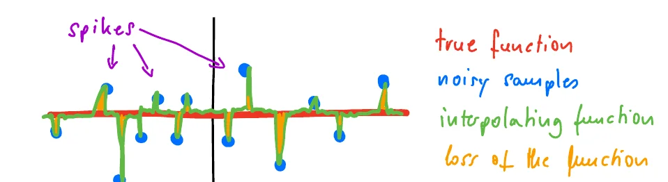
Slide 58: the interpolating function (green) follows the true function (red) and reaches each noisy sample (blue) with a narrow spike. The loss (orange) is only large inside the spikes.

Large spikes interpolate the noisy labels $y_i$; in high dimensions these regions have vanishing volume. Outside the spikes the function approximates the true function (here the 0 function). The maths in six steps:

1. Form of the prediction function. The solution lies in the span of the data points, so $f(x)={\sum }_{i=1}^n{\alpha }_i⟨x,x_i⟩$.
2. It interpolates. At the training points it takes the (potentially large) values $y_i$.
3. The spike. The region around a training point where $f$ is still large:

$$S_i(t)=\{x\in {\mathbb{R}}^d:⟨\frac{x}{\Vert x\Vert },\frac{x_i}{\Vert x_i\Vert }⟩>t\},$$

the set of points whose normalized projection onto $x_i$ exceeds $t$. 4. Concentration of random projections. In high dimensions random projections are highly concentrated. For $u,v$ drawn uniformly from the unit sphere in ${\mathbb{R}}^d$:

$$P(⟨u,v⟩>t)\le 2\exp (-cd{t}^2)$$

with a constant $c$. 5. The volume of the spikes is small. Union bound over the $n$ spikes:

$$P(x\in \bigcup _{i=1}^n{S}_i(t))\le 2n\exp (-cd{t}^2).$$

This explains why the spikes do not hurt consistency: if $n/d\to 0$, the error bound in the theorem goes to 0. 6. Outside the spikes the function is close to 0. In high dimensions the data points are nearly orthogonal. The function must be large at the training points to interpolate; this is possible because each point essentially “opens up” a new dimension, and there are enough parameters to memorize it there. A random test point is with high probability not aligned with any training point, so it lies outside the spikes. And because we take the minimum norm solution, the function has small norm in all directions without training points, so the prediction there is close to 0.

Why the minimum norm matters

An arbitrary interpolator could put large values anywhere in the $d-n$ directions that the data never sees. The minimum norm solution puts nothing there ($w_{\perp }=0$ from Theorem 1: GD finds the minimum norm solution). So it is spiky exactly at the data and flat everywhere else.

Memory aid

Spiky at the data, smooth everywhere else. In high dimensions the spikes are thin needles: almost no test point hits one.

Task: the spikes have vanishing volume

Exam-style task: spiky-smooth interpolation (4 P)

Math: union bound · logs

Use $P(x\in {\bigcup }_i{S}_i(t))\le 2n\exp (-cd{t}^2)$ with $c=\frac{1}{2}$, and spikes of width $t=0.2$.

(a) (1 P, easy) Evaluate the bound for $n=1000$ training points in $d=1000$ dimensions.

(b) (1.5 P, harder) For $n=1000$, from which dimension on is the probability of landing in a spike guaranteed to be at most $1\%$? How does this change if $n$ is multiplied by 10?

(c) (1.5 P, transfer) Theorem 3 (benign overfitting in the toy setup) gives the risk ${\sigma }^{2}n/(d-n-1)$. Which dimension is needed for $n=1000$ so that the risk is at most $1\%$ of ${\sigma }^2$? Compare with (b): which effect limits benign overfitting, the volume of the spikes or the variance?

Solution

(a) $2\cdot 1000\cdot \exp (-\frac{1}{2}\cdot 1000\cdot 0.04)=2000e^{-20}\approx 2000\cdot 2.06\cdot 10^{-9}\approx 4.1\cdot 10^{-6}$. (1 P)

(b) $2000e^{-0.02d}\le 0.01⟺e^{-0.02d}\le 5\cdot 10^{-6}⟺d\ge \ln (2\cdot 10^5)/0.02=12.21/0.02\approx 610.3$, so $d\ge 611$. With $n=10,000$: $d\ge \ln (2\cdot 10^6)/0.02=14.51/0.02\approx 725.4$, so $d\ge 726$. The required dimension grows only logarithmically in $n$. (1.5 P)

(c) $\frac{n}{d-n-1}\le 0.01⟺d\ge 101n+1=101,001$. The dimension must grow linearly in $n$ (that is the condition $n/d\to 0$). The spikes are already negligible at $d\approx 611$, but interpolation needs $d>n$ anyway, and a small variance needs $d\gg n$: the variance term is the binding constraint. (1.5 P)

Not so benign: isotropic Gaussian inputs

Slides 64-68

(Literature: Bach, Sec. 12.2.3; Bartlett, Long, Lugosi, Tsigler 2020; Bartlett, Montanari, Rakhlin 2021.)

Do similar results hold for linear regression with a real signal? Partially yes, but with caveats.

Setup: linear model, isotropic Gaussian sampling

• Inputs $x_1,\dots ,x_n\sim \mathcal{N}(0,I_d)$ i.i.d.
• Responses $y_i=x_i^{\top }{\theta }^{\ast }+{\epsilon }_i$ with the true signal ${\theta }^{\ast }\in {\mathbb{R}}^d$ and ${\epsilon }_i\sim \mathcal{N}(0,{\sigma }^2)$ i.i.d. (overall $\epsilon \sim \mathcal{N}(0,{\sigma }^2{I}_n)$).
• Design matrix $X\in {\mathbb{R}}^{n\times d}$, empirical covariance $\hat{\Sigma }=\frac{1}{n}{X}^{\top }X$.
• Excess risk at a test point: $R(\hat{\theta })=E_x(({\hat{\theta }}^{\top }x-{\theta }^{\ast \top }x{)}^2)$, then averaged over the training data: $E_{X,y}R(\hat{\theta })$.

Theorem 4 (expected excess risk, linear model, Gaussian data)

• Under-parameterized regime $n>d+1$ (OLS):

$$E_{X,y}R(\hat{\theta })=\underset{\text{variance}}{\underbrace{\frac{{\sigma }^{2}d}{n-d-1}}}$$

• Over-parameterized regime $d>n+1$ (minimum norm interpolator):

$$E_{X,y}R(\hat{\theta })=\underset{\text{variance}}{\underbrace{\frac{{\sigma }^{2}n}{d-n-1}}}+\underset{\text{bias}}{\underbrace{\Vert {\theta }^{\ast }{\Vert }^2\frac{d-n}{d}}}$$

Slide 68: excess risk (blue) against d. Left of n only variance; right of n the variance (falling) and the bias (rising) add up.

In particular:

• The variance terms are nice in both regimes (they look alike with the roles of $d$ and $n$ switched) and small far from the threshold.
• In the under-parameterized regime the estimate is unbiased.
• The bias in the over-parameterized regime does not explode (good), but it remains large unless we make strong assumptions.
• Here we would not say that benign overfitting takes place. Learning works better in the under-parameterized regime.

Proof of Theorem 4

Slides 69-85

Step 1: excess risk as a weighted norm.

$$R(\hat{\theta })=E_x((\hat{\theta }-{\theta }^{\ast }{)}^{\top }x{x}^{\top }(\hat{\theta }-{\theta }^{\ast }))=(\hat{\theta }-{\theta }^{\ast }{)}^{\top }\Sigma (\hat{\theta }-{\theta }^{\ast })=:\Vert \hat{\theta }-{\theta }^{\ast }{\Vert }_{\Sigma }^2,\Sigma =E(x{x}^{\top }).$$

Step 2: bias-variance decomposition. Since $y$ is a deterministic function plus noise, the expectation over $y$ is one over $\epsilon$:

$$E_{X,\epsilon }\Vert \hat{\theta }-{\theta }^{\ast }{\Vert }_{\Sigma }^2=\underset{\text{bias}}{\underbrace{E_X\Vert E_{\epsilon }(\hat{\theta }\mid X)-{\theta }^{\ast }{\Vert }_{\Sigma }^2}}+\underset{\text{variance}}{\underbrace{E_{X,\epsilon }\Vert \hat{\theta }-E_{\epsilon }(\hat{\theta }\mid X){\Vert }_{\Sigma }^2}}.$$

Step 3: under-parameterized, $n\ge d+2$. The estimator is OLS, $\hat{\theta }=(X^{\top }X{)}^{-1}{X}^{\top }y$, unbiased. From the random design result (Lecture 5) the excess risk is $\frac{{\sigma }^2}{n}E\mathrm{tr}(\Sigma {\hat{\Sigma }}^{-1})$ with $\Sigma =I_d$ and ${\hat{\Sigma }}^{-1}=n(X^{\top }X{)}^{-1}$, i.e. ${\sigma }^{2}E\mathrm{tr}(X^{\top }X{)}^{-1}$. $X^{\top }X$ is Wishart with $n$ degrees of freedom, $E((X^{\top }X{)}^{-1})=I_d/(n-d-1)$, so the risk is ${\sigma }^{2}d/(n-d-1)$. For $d\ll n$ it is small.

Step 4: at the threshold, $n\approx d$. For $n=d$ and $n=d+1$, $E\mathrm{tr}(X^{\top }X{)}^{-1}=\infty$ (a property of Wishart matrices with $d$ or $d+1$ degrees of freedom). The variance explodes: this is why the double descent plot diverges at $d=n$.

Step 5: over-parameterized, $n<d$, intuition. The signal lives in $d$ dimensions but we have $n\ll d$ points. Even if each point identified one parameter of ${\theta }^{\ast }$ perfectly, we could not observe all $d$ directions. So in general the risk does not become small. That would need assumptions saying that ${\theta }^{\ast }$ is described by at most order $n$ parameters. GD/SGD converges to $\hat{\theta }=X^{\top }(X{X}^{\top }{)}^{-1}y$.

Step 6: variance term. $\hat{\theta }=X^{\top }(X{X}^{\top }{)}^{-1}(X{\theta }^{\ast }+\epsilon )=X^{\top }(X{X}^{\top }{)}^{-1}X{\theta }^{\ast }+X^{\top }(X{X}^{\top }{)}^{-1}\epsilon$ and $E_{\epsilon }(\epsilon \mid X)=0$, so $E_{\epsilon }(\hat{\theta }\mid X)=X^{\top }(X{X}^{\top }{)}^{-1}X{\theta }^{\ast }$ and $\hat{\theta }-E_{\epsilon }(\hat{\theta }\mid X)=X^{\top }(X{X}^{\top }{)}^{-1}\epsilon$. With $\Sigma =I$:

$$E\Vert X^{\top }(X{X}^{\top }{)}^{-1}\epsilon {\Vert }^2=E({\epsilon }^{\top }(X{X}^{\top }{)}^{-1}X{X}^{\top }(X{X}^{\top }{)}^{-1}\epsilon )=E({\epsilon }^{\top }(X{X}^{\top }{)}^{-1}\epsilon )={\sigma }^{2}E\mathrm{tr}(X{X}^{\top }{)}^{-1}={\sigma }^2\frac{n}{d-n-1},$$

the same term as in the toy setup. It goes to 0 as $d\to \infty$ with $n/d\to 0$.

Step 7: bias term. The noise part vanishes in expectation, so with $\Sigma =I$:

$$E_X\Vert X^{\top }(X{X}^{\top }{)}^{-1}X{\theta }^{\ast }-{\theta }^{\ast }{\Vert }^2=E_X{\theta }^{\ast \top }(I-X^{\top }(X{X}^{\top }{)}^{-1}X){\theta }^{\ast }.$$

$P:=X^{\top }(X{X}^{\top }{)}^{-1}X\in {\mathbb{R}}^{d\times d}$ is a projection ($P^2=P$) onto the random $n$-dimensional subspace $\mathrm{range}(X^{\top })$: it maps every data point to itself and every vector in $\ker X$ to 0. Because the data is $\mathcal{N}(0,I)$, this subspace is uniformly distributed, so we may rotate and replace ${\theta }^{\ast }$ by $\Vert {\theta }^{\ast }\Vert e_j$ for any $j$, and average over all $j$:

$$E{\theta }^{\ast \top }P{\theta }^{\ast }=\Vert {\theta }^{\ast }{\Vert }^2\cdot \frac{1}{d}\sum _{j=1}^{d}E{e}_j^{\top }P{e}_j=\Vert {\theta }^{\ast }{\Vert }^2\cdot \frac{E\mathrm{tr}(P)}{d}=\Vert {\theta }^{\ast }{\Vert }^2\frac{n}{d},$$

using ${\sum }_j{e}_j^{\top }A{e}_j=\mathrm{tr}A$ and that the trace of a projection onto an $n$-dimensional subspace is $n$ (or cyclicity: $\mathrm{tr}(X^{\top }(X{X}^{\top }{)}^{-1}X)=\mathrm{tr}(I_n)=n$). So the bias is $\Vert {\theta }^{\ast }{\Vert }^2-\Vert {\theta }^{\ast }{\Vert }^2\frac{n}{d}=\Vert {\theta }^{\ast }{\Vert }^2\frac{d-n}{d}$. $\square$

What the bias term means (slide 85)

• If ${\theta }^{\ast }=0$, the bias is 0: that is the toy setup, benign overfitting.
• If ${\theta }^{\ast }\ne 0$: for $n\ll d$ the factor $(d-n)/d$ is of order 1. It does not vanish; we cannot recover the true model. Intuitively, with $n$ points we only capture an $n/d$ fraction of the signal, the rest “gets lost”. We interpolate, but a large bias remains: not benign overfitting in general.

Task: evaluating Theorem 4 (excess risk in both regimes)

Exam-style task: under vs. over-parameterized (4 P)

Math: bias and variance

Isotropic Gaussian inputs, $n=100$, ${\sigma }^2=1$, $\Vert {\theta }^{\ast }{\Vert }^2=1$.

(a) (1 P, easy) Compute the expected excess risk for $d=20$ and for $d=90$.

(b) (1.5 P, harder) Compute variance, bias and excess risk of the minimum norm interpolator for $d=200$, $d=1000$ and $d=10,000$.

(c) (1.5 P, transfer) Compare with the trivial predictor $\hat{\theta }=0$. Is this benign overfitting? What changes if ${\theta }^{\ast }=0$?

Solution

(a) $d=20$: $\frac{20}{100-20-1}=\frac{20}{79}\approx 0.25$. $d=90$: $\frac{90}{9}=10$: close to the threshold the variance blows up. (1 P)

(b)

$d$	variance $\frac{n}{d-n-1}$	bias $\frac{d-n}{d}$	excess risk
200	$100/99\approx 1.010$	$0.5$	$\approx 1.51$
1000	$100/899\approx 0.111$	$0.9$	$\approx 1.01$
10,000	$100/9899\approx 0.010$	$0.99$	$\approx 1.00$

The variance vanishes, the bias grows to $\Vert {\theta }^{\ast }{\Vert }^2=1$. (1.5 P)

(c) $\hat{\theta }=0$ has excess risk $\Vert 0-{\theta }^{\ast }{\Vert }_{\Sigma }^2=\Vert {\theta }^{\ast }{\Vert }^2=1$. For $d\gg n$ the interpolator is no better than predicting 0, and the under-parameterized model with $d=20$ is much better (0.25). Not benign. With ${\theta }^{\ast }=0$ only the variance remains (0.111 and 0.010 for $d=1000$ and $10,000$): that is Theorem 3 (benign overfitting in the toy setup), benign. (1.5 P)

Benign overfitting with an aligned covariance

Slides 86-95

(Literature: Bartlett, Montanari, Rakhlin, “Deep learning: a statistical viewpoint”, Acta Numerica 2021.)

More general setup

• Inputs $x_i$ from some distribution on ${\mathbb{R}}^d$ with $E(x_i)=0$ and covariance $\Sigma =E(x{x}^{\top })=\mathrm{diag}({\lambda }_1,\dots ,{\lambda }_d)$, ${\lambda }_1\ge {\lambda }_2\ge \cdots \ge {\lambda }_d$. W.l.o.g. the eigenvectors are the unit vectors $e_1,\dots ,e_d$ in this order.
• Linear truth $f^{\ast }(x)=⟨{\theta }^{\ast },x⟩$; over-parameterized, $d>n$.

There is not enough data to learn all $d$ directions of ${\theta }^{\ast }$. It becomes possible only if the covariance has a nice structure that separates the directions used for learning the signal from the directions used for interpolating the noise.

Theorem 5 (excess risk of the minimum norm interpolator, general case)

Let $\hat{\theta }=X^{\top }(X{X}^{\top }{)}^{-1}y$. Choose $k<d$ such that the tail is not dominated by only a few eigenvalues (details skipped). Then

$$ER(\hat{\theta })\lesssim \underset{\text{bias: loss from directions not learned}}{\underbrace{\sum _{i=1}^d{\lambda }_i{\theta }_i^{\ast 2}{\left(\frac{\frac{1}{n}{\sum }_{j>k}{\lambda }_j}{{\lambda }_i+\frac{1}{n}{\sum }_{j>k}{\lambda }_j}\right)}^2}}+\underset{\text{variance: cost of fitting the noise}}{\underbrace{{\sigma }^2\left(\frac{k}{n}+\frac{n{\sum }_{i>k}{\lambda }_i^2}{({\sum }_{i>k}{\lambda }_i{)}^2}\right)}}$$

The proof is difficult (papers by Bartlett et al.), we skip it and look at the two terms separately.

Variance term. ${\sigma }^2(\frac{k}{n}+n\frac{{\sum }_{i>k}{\lambda }_i^2}{({\sum }_{i>k}{\lambda }_i{)}^2})$: the first part is the variance in the signal itself, the second the tail weight from the interpolation part. It depends on the input covariance and on $\sigma$, not on ${\theta }^{\ast }$. It is small if the tail has many small eigenvalues and large if it has one (or few) dominant tail eigenvalues:

• Flat tail ${\lambda }_{k+1}=\cdots ={\lambda }_d=a$: $n\frac{(d-k)a^2}{((d-k)a{)}^2}=\frac{n}{d-k}$. For small $k$, small $n$ and large $d$ this is small. Good.
• One tail eigenvalue ${\lambda }_{k+1}=a$, all others 0: $n\frac{a^2}{a^2}=n$, which does not vanish. Bad.

Bias term. With ${\theta }_i^{\ast }$ the signal strength along eigenvector $e_i$, the bias is roughly ${\sum }_i{\lambda }_i{\theta }_i^{\ast 2}(\frac{r}{{\lambda }_i+r}{)}^2$ with $r=\frac{1}{n}{\sum }_{j>k}{\lambda }_j$:

• Signal aligned with the top eigenvectors: the covariance mainly lives in the first dimension (${\lambda }_1\gg {\sum }_{j>k}{\lambda }_j$, and that tail sum is small) and ${\theta }^{\ast }=e_1$. All terms but the first vanish, and the first is small because $r\ll {\lambda }_1$. Good.
• Signal in the tail: ${\theta }_1^{\ast }=\cdots ={\theta }_k^{\ast }=0$ and the remaining ${\theta }_j^{\ast }$ large. The first $k$ terms vanish, the others are large because ${\lambda }_i$ is small compared to $r$. Bad.

Good and bad situations (slides 94-95)

Good (benign overfitting): the spectrum has few large eigenvalues ${\lambda }_1,\dots ,{\lambda }_k$ and then many tiny ones, and ${\theta }^{\ast }$ is aligned with the top eigenvalues. Signal and data essentially live in the same $k$-dimensional subspace, so bias and variance are both small. The top $k$ directions represent the signal (like the under-parameterized regime), the remaining $d-k$ directions interpolate the noise without accumulating bias.

Bad:

• The tail has too much weight: bias accumulates. The interpolator catches only an $n/d$ fraction of the signal and $1-n/d$ noise (the isotropic $\mathcal{N}(0,I)$ case above).
• The tail has few dominant eigenvalues: the variance does not go to 0.
• ${\theta }^{\ast }$ is not aligned with the dominating eigenvalues: the bias does not go to 0, there is not enough data to learn the signal.

Memory aid

A few loud directions carry the signal, many quiet ones soak up the noise. Too few quiet ones: variance. Too many loud ones or signal in the quiet ones: bias.

Four regimes in a Fourier example

Slides 96-102

A toy example that shows the behavior:

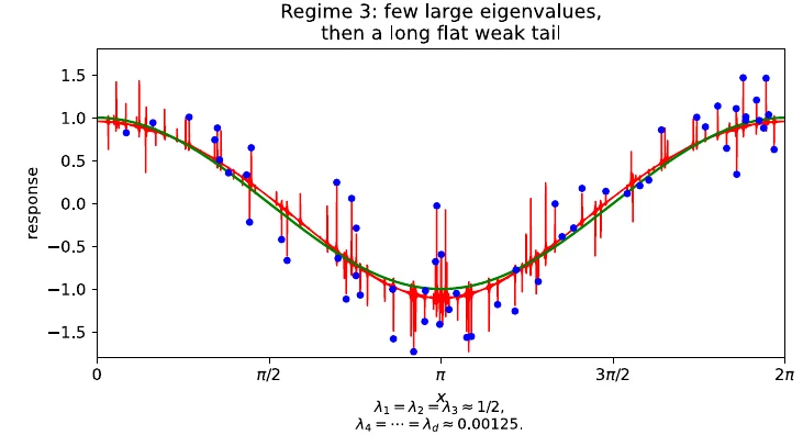
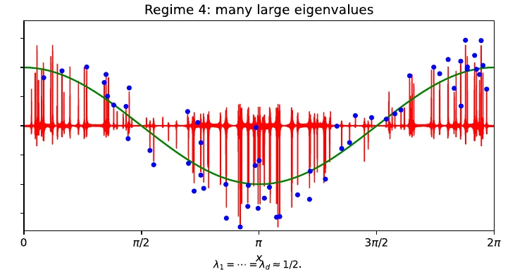
• $n=60$ points uniform on $[0,2\pi ]$, represented in a Fourier basis ${\phi }_j(x)=s_j\cos (jx)$ in dimension $d=2000$ (different $s_j$ below).
• The eigenvectors of the true covariance are the basis vectors, so the covariance is diagonal with eigenvalues ${\lambda }_i=s_i^2/2$.
• True function $\cos (x)$, the first basis function: ${\theta }^{\ast }=(1,0,\dots ,0)$, always perfectly aligned with the first eigenvector.
• Noisy outputs $y_i=\cos (x_i)+{\epsilon }_i$ with ${\epsilon }_i\sim \mathcal{N}(0,0.01)$; we look at the minimum norm interpolator. Plots: true function green, data blue, minimum norm solution red.

Regime	Spectrum	Behavior
1	few large eigenvalues, then many 0	like the under-parameterized regime: no interpolation possible, but learning works if the signal is aligned with the covariance
2	few large, then few small ones	interpolation possible once there are enough small tail eigenvalues (essentially $n$ non-zero ones), but the variance stays large; it decreases with the number of small non-zero eigenvalues
3	few large, many small ones	benign overfitting
4	many large eigenvalues	impossible to learn, bias remains high (essentially the isotropic Gaussian case)

Slide 100, regime 3: few large eigenvalues and a long flat tail. The fit follows cos(x) and only spikes at the points.

Slide 101, regime 4: many large eigenvalues. The fit interpolates but is pulled towards 0 away from the data: the signal is lost.

Explore: the four regimes and the double descent formula

Top: the Fourier example of slides 96-101, recomputed live (n = 60, d = 2000, noise variance 0.01). Presets for the four regimes; the sliders change the number of large eigenvalues, the tail length and the tail height. Bottom: Theorem 4 (excess risk in both regimes) as a function of d, with variance and bias.

Things to try: in regime 2 move the tail length from 57 to 147 to 1997 and watch the variance (the wild oscillations) shrink. In regime 3 raise the tail height: the tail steals weight from the signal, the fit flattens (bias). In the lower plot set the signal to 0: only the variance is left, and the curve goes to 0 for large d (Theorem 3: benign overfitting in the toy setup).

Summary for linear regression (slide 102)

Whether benign overfitting can take place depends on the covariance matrix of the data and whether it is aligned with the signal ${\theta }^{\ast }$. It can happen if the effective dimension $k$ of the signal is small compared to $n$ and the remaining dimensions contain isotropic small noise that allows the interpolation. The analysis is difficult, and little is known beyond the linear setting.

Task: which spectrum is benign?

Exam-style task: reading the terms of Theorem 5, the excess risk for a general covariance (4 P)

Math: eigenvalues of a covariance

$n=50$, ${\sigma }^2=0.04$, signal ${\theta }^{\ast }=e_1$, $k=2$ large eigenvalues ${\lambda }_1={\lambda }_2=1$.

(a) (1 P, easy) Compute the variance term for a flat tail of $d-k=5000$ eigenvalues $a=0.001$.

(b) (1.5 P, harder) Compute the variance term for a tail with only one non-zero eigenvalue $a=0.001$, and for a flat tail of $d-k=100$ eigenvalues. Rank the three spectra.

(c) (1.5 P, transfer) For the flat tail of (a), compute the bias term. Then assume the signal is ${\theta }^{\ast }=e_{10}$, a tail direction with ${\lambda }_{10}=0.001$. What fraction of this signal is lost?

Solution

(a) Flat tail: $n\frac{\sum {\lambda }_i^2}{(\sum {\lambda }_i{)}^2}=\frac{n}{d-k}=\frac{50}{5000}=0.01$. Variance $=0.04(\frac{2}{50}+0.01)=0.04\cdot 0.05=0.002$. (1 P)

(b) One tail eigenvalue: $n\frac{a^2}{a^2}=n=50$, variance $0.04(0.04+50)\approx 2.0$, bad. Flat tail of 100: $\frac{50}{100}=0.5$, variance $0.04\cdot 0.54=0.0216$. Ranking: 5000-tail ($0.002$) < 100-tail ($0.022$) < single tail eigenvalue ($2.0$). The longer and flatter the tail, the smaller the cost of fitting the noise. (1.5 P)

(c) $r=\frac{1}{n}{\sum }_{j>k}{\lambda }_j=\frac{5000\cdot 0.001}{50}=0.1$. Only $i=1$ contributes: ${\lambda }_1(\frac{r}{{\lambda }_1+r}{)}^2=1\cdot (0.1/1.1{)}^2\approx 0.0083$, small compared to the signal variance ${\lambda }_1=1$: bias and variance small, benign. For ${\theta }^{\ast }=e_{10}$: $(\frac{r}{{\lambda }_{10}+r}{)}^2=(0.1/0.101{)}^2\approx 0.98$, so about 98% of the signal ${\lambda }_{10}{\theta }_{10}^{\ast 2}$ is lost: the signal is not aligned with the top eigenvalues, bad. (1.5 P)

Does benign overfitting contradict classical learning theory?

Slides 103-108

(Literature: Zhou, Sutherland, Srebro, “On uniform convergence and low-norm interpolation learning”, NeurIPS 2020.)

Hang on: the function classes of deep learning are so large that classical generalization bounds are not informative. But Vapnik’s theorem (Lecture 3) says uniform convergence is not only sufficient but also necessary for consistency. Where is the catch?

The catch

• The function class a network can represent is huge, but we select the solution from a tiny subset of it (implicit regularization).
• For the minimum norm interpolator in linear regression, Zhou, Sutherland and Srebro (2020) prove that the set of functions of small norm is still too large for uniform convergence: “uniformly bounding the difference between empirical and population errors cannot show any learning in the norm ball, and cannot show consistency for any set, even one depending on the exact algorithm and distribution.”
• But uniform convergence can be proven if one further restricts to functions that have a small norm and interpolate. See also Shamir, “The implicit bias of benign overfitting”, 2022.

Summary of "modern" learning theory (slides 106-108)

The current chain of arguments for why deep networks generalize:

1. Consider the highly over-parameterized, high-dimensional setting.
2. By the geometry of the loss landscape, SGD (or other algorithms) finds global optima, i.e. interpolating solutions, easily.
3. Under certain conditions, implicit regularization gives this solution nice properties (e.g. minimum norm).
4. For such solutions one can prove generalization under certain assumptions (e.g. through the simple-plus-spiky decomposition).

This explains why deep networks might work. It does not explain whether we need them: perhaps we just haven’t found a simpler approach. Perhaps not: the arguments on smooth interpolation show that robust solutions need large models (not necessarily networks, but models with many parameters). Many results hold only in special cases under special assumptions; none has been extended to the really interesting scenarios yet.

Why do we need large models?

Representation power of neural networks

Slides 111-118

Two very different questions:

• Representation power: which functions can a specific network represent at all? How can we describe this function space mathematically?
• Trainability: if a network can represent a function and we observe training data from it, can we actually find a parameter vector that represents it?

Networks with one hidden layer with $m$ units, continuous activation $\sigma$ and one linear output neuron represent the family

$$\mathcal{F}:=\mathrm{span}\{x\mapsto \sigma (w^{\top }x+b):w\in {\mathbb{R}}^d,b\in \mathbb{R}\}.$$

Theorem 6 (universal approximation; Pinkus, Acta Numerica 1999)

Let $K\subset {\mathbb{R}}^d$ be compact. If the activation $\sigma$ is continuous and not a polynomial, then $\mathcal{F}$ is dense in $C(K)$ (continuous functions, sup-norm): for every $f^{\ast }\in C(K)$ and every $\epsilon >0$ there are a number $m$ of hidden units and parameters $\theta$ with

$$\underset{x\in K}{\sup }|f^{\ast }(x)-f_{\theta }(x)|<\epsilon .$$

Proof sketch of Theorem 6

Case 1: $\sigma \in C^{\infty }(\mathbb{R})$.

• Derivatives of a neuron with respect to $w$ lie in $\bar{\mathcal{F}}$ (the closure). Fix $w$, $b$, $i$ and take the difference quotient

$$Q_h(x)=\frac{\sigma ((w+h{e}_i{)}^{\top }x+b)-\sigma (w^{\top }x+b)}{h}.$$

For each $h\ne 0$, $Q_h$ is a linear combination of two neurons, so $Q_h\in \mathcal{F}$ and ${\lim }_{h\to 0}{Q}_h={\partial }_{w_i}\sigma (w^{\top }x+b)\in \bar{\mathcal{F}}$.

• Extending this to every multi-index $\alpha =({\alpha }_1,\dots ,{\alpha }_d)$: $\frac{{\partial }^{|\alpha |}}{\partial w^{\alpha }}\sigma (w^{\top }x+b)=x^{\alpha }{\sigma }^{(|\alpha |)}(w^{\top }x+b)\in \bar{\mathcal{F}}$ with $x^{\alpha }:=x_1^{{\alpha }_1}\cdots x_d^{{\alpha }_d}$.
• Set $w=0$: $x^{\alpha }{\sigma }^{(|\alpha |)}(b)\in \bar{\mathcal{F}}$ for every $b$. Because $\sigma$ is not a polynomial, for each $k$ there is $b_k$ with ${\sigma }^{(k)}(b_k)\ne 0$; dividing by it gives $x^{\alpha }\in \bar{\mathcal{F}}$.
• So $\bar{\mathcal{F}}$ contains all monomials, hence all polynomials, and by the Weierstrass theorem polynomials are dense in $C(K)$.

Case 2: $\sigma \notin C^{\infty }$. Smooth it first (e.g. convolution with a $C^{\infty }$ function) and adapt the argument. $\square$

What universal approximation does not say

So two-layer networks suffice for pretty much everything? Yes, but the theorem says nothing about

• how large $m$ must be depending on $\epsilon$ and the complexity of $f^{\ast }$,
• the complexity of the solution $f_{\theta }$ (e.g. its Lipschitz constant),
• whether such a function can be found from training data, and how much data it needs,
• generalization outside the training set.

Depth can be more expressive than width (Telgarsky, COLT 2016): fix a depth $L$. There is a function $f_L$ exactly represented by a ReLU network of depth $L$ and width $O(1)$, but approximating it with depth at most $L-1$ up to constant accuracy (in $L_1$) needs width of order $2^{\Omega (L)}$.

Gradient descent might not learn a small network

Slides 119-122

Is it always easy to find a function that a network can represent? There are negative results. Setup:

• A “nice” input distribution $D$ on ${\mathbb{R}}^d$ (uniform on $\{-1,+1{\}}^d$, standard Gaussian, uniform on the sphere).
• Any architecture $f_{\theta }$ with $\mathrm{poly}(d)$ parameters (a “small” network).
• An idealized learner that queries the gradient of the true population loss, ${\nabla }_{\theta }{E}_{x\sim D}\ell (f_{\theta }(x),f^{\ast }(x)){|}_{\theta ={\theta }_t}$, and runs GD, SGD, Adam, … from some ${\theta }_0$. No finite-sample and no computational issues.

Theorem 7 (hardness of learning a simple network; Shamir, JMLR 2018)

There is a family $\mathcal{F}$ of targets $f^{\ast }:{\mathbb{R}}^d\to \mathbb{R}$ such that

1. every $f^{\ast }\in \mathcal{F}$ is exactly computed by $f_{\theta }$ for some ${\theta }^{\ast }$ (a small network suffices), and
2. any (randomized, computationally unbounded) algorithm that sees the data only through $T$ (possibly noisy) gradient queries and outputs $\hat{f}$ with $P_x(\hat{f}(x)\ne f^{\ast }(x))\le \frac{1}{3}$ for a uniformly random $f^{\ast }\in \mathcal{F}$ must use $T\ge 2^{\Omega (d)}$ queries.

So a small network exists, but no gradient-based algorithm finds it in polynomial time. Representation is not the whole story: we need to look at specific algorithms to understand what they can and cannot learn.

Large models are necessary for robust interpolation

Slides 123-130

(Literature: Bubeck and Selke, “A universal law of robustness via isoperimetry”, NeurIPS 2021; extended version Journal of the ACM 2023.)

Robustness means a function that is “not too wiggly”, measured by the Lipschitz constant

$$L(f):=\underset{x,y}{\max }\frac{|f(x)-f(y)|}{\Vert x-y\Vert }.$$

The higher $L(f)$, the less robust. Ideally $L$ is a constant that does not depend on $n$ or $d$.

Interpolation: to solve $n$ equations you typically need only $n$ unknowns, but that solution can have a very high Lipschitz constant. A larger function class has more interpolating solutions; is there one with a low Lipschitz constant? Empirically, larger networks help tremendously for robustness.

Result by Bubeck and Selke (in words)

Let $\mathcal{F}$ be smoothly parameterized by $p$ parameters and the $d$-dimensional data come from a somewhat nice distribution. Then any function in $\mathcal{F}$ that fits the training data below the noise level (e.g. interpolates) must have

$$L(f)\gtrsim \sqrt{\frac{nd}{p}}.$$

Conversely, for Lipschitz constant $L=1$ we need $p\gtrsim nd$ parameters.

• Construction showing $nd$ suffices: uniform distribution on the unit sphere in ${\mathbb{R}}^d$, $n$ random points (moderate $n$). With probability at least $1-\exp (-\Omega (d))$ any two points are at distance at least 1 (concentration). Choose any labels and put a “bump” $g$ (some RBF) on every point: $f(x)={\sum }_{i=1}^{n}g(\Vert x-x_i\Vert )y_i$. It interpolates, has Lipschitz constant 1 and needs $d\cdot n$ parameters (the $n$ centers).
• Proof idea for a finite class of $N$ functions with Lipschitz constant $L$: by concentration, a fixed $f$ fits $n$ random labels with probability at most $\exp (-nd/L^2)$. Union bound: some $f\in \mathcal{F}$ fits with probability at most $N\exp (-nd/L^2)=\exp (\log N-nd/L^2)$. This only becomes large if $L$ is of order $\sqrt{nd/\log N}$: any interpolating function must have $L$ at least of that order. For infinite classes an $\epsilon$-net argument replaces $\log N$ by $p$. The results extend to generalization bounds.
• ImageNet: the authors estimate that a robust estimator needs of the order $10^{11}$ parameters (models in 2021 had about $10^9$). If correct, robust ImageNet classification is only a matter of time: no new tools, just larger models.

Mini example with own numbers

$n=10^4$ training points in $d=100$ dimensions. For $L=1$: $p\gtrsim nd=10^6$ parameters. A model with only $p=n=10^4$ parameters can interpolate, but then $L\gtrsim \sqrt{10^6/10^4}=10$. With $p=2.5\cdot 10^5$: $L\gtrsim \sqrt{4}=2$. Doubling robustness (halving $L$) costs four times the parameters.

The loss landscape in our favor

Slides 132-139

Minimizing a loss over a complex network is typically not convex, yet standard optimizers do a surprisingly good job at finding good local or even global optima. Some hypotheses why (not explored in depth; many results hold only for specific architectures and losses):

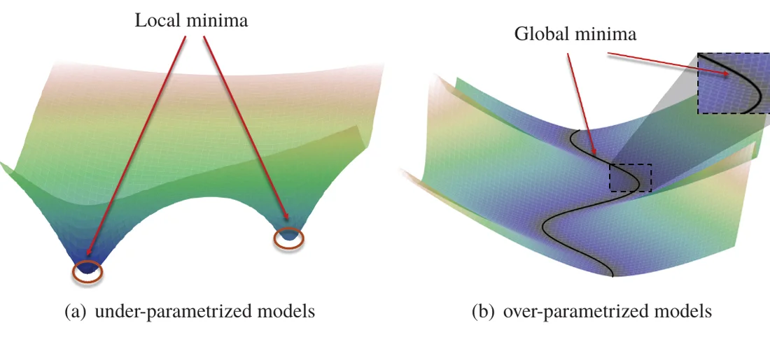
Slide 133: (a) under-parameterized: isolated local minima, the result depends on the start. (b) over-parameterized: a connected manifold of global minima (Belkin 2021).

• Why SGD finds a global optimum: we expected non-convex problems to look like the left picture (lots of local optima). In the over-parameterized regime they rather look like the right one: no matter where we start, we end in a global minimum, and there are many of them. This can be characterized and proved (Belkin 2021 and references).
• Many connected global minima: with $m$ parameters and $n$ points, $m>n$, the set of global minima is usually not discrete but an $(m-n)$-dimensional submanifold (Cooper, 2018). Making a network wider can connect previously discrete minima into one manifold (Simsek et al., ICML 2021).
• Low-loss paths: the minima found by two networks are connected by a path of non-increasing error (Frankle et al., ICML 2020, linear mode connectivity).
• Width removes bad basins: from narrow to wide networks there is a phase transition from suboptimal basins to none (Li, Tang, Sun, SIAM J. Optimization 2022). Over-parameterized deep networks have no strict local minima for any continuous activation (Li, Ding, Sun): the landscape can have bad plateaus, but no strict bad basin.
• Training dynamics, e.g. edge of stability: one might expect large learning rates to push training toward flatter solutions because sharp regions are unstable. Instead GD often sits right at the maximum sharpness compatible with the step size (Cohen, Damian, Talwalkar, Kolter, Lee, ICLR 2025; blog: centralflows.github.io).
• Architecture matters: skip connections make the loss landscape smoother (Li et al., “Visualizing the loss landscape of neural nets”, NeurIPS 2018, ResNet-56 with and without skip connections).

Summary

Many papers show that for certain architectures, losses and optimizers something nice happens. General tenor: a large number of parameters helps. Many papers also explain tricks of the trade through the landscape. There is no single reason that explains the success of network optimization, but together the results paint a picture.

Infinite width theory and the neural tangent kernel

Slides 140-147

(Literature: Jacot, Gabriel, Hongler, “Neural tangent kernel”, NeurIPS 2018; Arora, Du, Hu, Li, Salakhutdinov, Wang, “On exact computation with an infinitely wide neural net”, NeurIPS 2019; Chizat, Oyallon, Bach, “On lazy training in differentiable programming”, NeurIPS 2019.)

A branch of theory studies wide shallow networks, e.g. one very wide hidden layer, to see why very wide networks might or might not be good.

Gradient flow is GD with infinitesimal step size (Bach, Sec. 12.3). Let $u_t=(f_{w_t}(x_1),\dots ,f_{w_t}(x_n){)}^{\top }\in {\mathbb{R}}^n$ be the predictions on the training points at time $t$. For a fully connected differentiable network trained with squared loss (Arora et al., Lemma 3.1):

$$\frac{d{u}_t}{dt}=-H_t(u_t-y),H_{ij,t}=⟨\frac{\partial f_{w_t}(x_i)}{\partial w},\frac{\partial f_{w_t}(x_j)}{\partial w}⟩.$$

$H_t\in {\mathbb{R}}^{n\times n}$ is an inner product matrix of gradients, i.e. a kernel matrix.

NTK regime and the neural tangent kernel

• For a two-layer ReLU network that is very wide, $H_t$ barely changes during training: $H_t\approx H_0$ (Arora et al., App. D).
• As the width goes to infinity, $H_0$ converges to a kernel function, the neural tangent kernel

$$K_{NTK}(x,x^{\prime })=⟨{\nabla }_{w}f(w_0,x),{\nabla }_{w}f(w_0,x^{\prime })⟩,$$

with $w_0$ the random initialization. It measures how similarly the predictions at $x$ and $x^{\prime }$ change under an infinitesimal parameter update.

• Consequence: in the infinite-width regime, training the network behaves like training a kernel method with $K_{NTK}$; the limiting solutions can be computed exactly for several losses.

No feature learning in the NTK regime

• In very wide networks every parameter changes only by a minuscule amount (lazy training): the gradient signal is spread over so many neurons that tiny changes add up to something substantial in the output, while the weights hardly move.
• So the network does not learn a new representation; it sticks to the random one from the initialization and behaves like a random feature model.
• In practice, networks trained in the lazy regime perform worse and do not exceed some classical linear methods.
• Limitations: the network stays close to its initialization, the tangent features stay essentially fixed, the model behaves like a kernel method, representation learning is largely absent. NTK theory explains optimization of very wide networks, but not feature learning as it happens in practical networks.

Theory regarding depth Slide 149: there are isolated results on very deep networks, but they are specific to individual architectures and do not tell a coherent story. Currently there is no convincing line of work explaining why networks need to be deep; it is a widely open research question.

Take home

Under- vs. over-parameterized learning

Slides 151-157

	Under-parameterized regime	Over-parameterized regime
setup	not so many data points	huge number of sample points
features	explicit prior knowledge: feature representation, similarity, distance, kernel	no explicit representation; features learned by the network (hard to interpret), raw pixels or tokens
training	control the capacity of the function class, be careful not to overfit	complex architecture, often trained to 0 training error and beyond
guiding principles	bias-variance decomposition, small function classes or regularization, stability; enforced explicitly	the same “old” principles at work implicitly: bias-variance beyond the interpolation threshold, implicit regularization by the algorithm, stability of the optimizers; analysis shifts from statistics to the optimization algorithm

Old principles in new disguise. On the downside: most theoretical results hold for rather simple models, and it is not proven that they hold in complex ones; there might be other powerful principles we haven’t identified. There is no magic involved, but it is sometimes hard to see behind the curtain. We are still very far from really understanding learning in the over-parameterized regime.

Which approach to use? Many applications still need the under-parameterized regime: there is not enough data to train a complex network. Neural networks are super-helpful when we have or can generate a lot of data (images, text, but also e.g. simulation-based inference in science). As an ML engineer you need to be confident in both worlds.

New failure modes

Deep learning shows failure modes that partly exist in the classical regime but are more pronounced now: adversarial examples, spurious features, shortcut learning, … Reasons: raw data without much pre-processing (hoping ML discovers whatever is needed), complex architectures that are hard to gain intuition about, black-box models that even ML engineers cannot understand. Together with the lack of strong theory: careful testing, benchmarking and validating play a central role now (see validity, Lecture 7).

Summary

Topic	Key message
puzzle	networks interpolate (even random labels) and still generalize; classical bounds vacuous
double descent	test error peaks at the interpolation threshold (parameters = data points) and can fall again; not always (polynomials), shape depends on how parameters are counted
implicit regularization	GD from 0 on least squares: $w^{\star }=X^{\top }(X{X}^{\top }{)}^{-1}y$, minimum norm; logistic GD on separable data: max-margin direction
benign overfitting, toy	${\theta }^{\ast }=0$: risk ${\sigma }^{2}n/(d-n-1)\to 0$; spiky-smooth, spikes of volume $\le 2n{e}^{-cd{t}^2}$
isotropic model	variance ${\sigma }^{2}n/(d-n-1)$ small, bias $\Vert {\theta }^{\ast }{\Vert }^2(d-n)/d$ stays; under-param: ${\sigma }^{2}d/(n-d-1)$; $\infty$ at $d\approx n$
aligned covariance	benign if few large eigenvalues carry the signal and a long flat tail of small ones absorbs the noise
classical theory	uniform convergence fails on the norm ball, holds on low-norm interpolating functions
large models	universal approximation; GD can need $2^{\Omega (d)}$ steps; robust interpolation needs $p\gtrsim nd$
landscape, NTK	many connected global minima; very wide nets are lazy, kernel-like, no feature learning

Self-Test

Question cards (13)

What is the interpolation threshold? Where is it for a random feature model, a polynomial regression and a one-hidden-layer classification network?

Answer

The model size from which training error 0 is possible, roughly as many parameters as equations. Random features: $m=n$. Polynomial of degree $d$: $d+1=n$, i.e. $d=n-1$. Network with $K$ outputs: about $n\cdot K$ parameters.

Why does the experiment with random labels challenge classical learning theory?

Answer

The network reaches training error 0 on randomly shuffled labels, so its shattering coefficient is maximal and VC or Rademacher bounds are vacuous. The same network generalizes on the real labels, which these bounds cannot explain.

Describe the double descent curve. Does it always occur?

Answer

Test error follows the classical U-curve, peaks at the interpolation threshold and decreases again in the over-parameterized regime, sometimes below the classical optimum. No: polynomial regression with monomials gets worse beyond the threshold, and single or triple descent also occur; the shape also depends on how parameters are counted.

State Theorem 1 (GD finds the minimum norm solution). Which assumptions does it need?

Answer

For $n<d$, $X$ of full row rank, GD on $\frac{1}{2}\Vert Xw-y{\Vert }^2$ from $w_0=0$ with $0<\eta <2/{\lambda }_{\max }(X{X}^{\top })$ converges to $w^{\star }=X^{\top }(X{X}^{\top }{)}^{-1}y$, the unique interpolating solution with minimal Euclidean norm.

Why are all GD iterates in the span of the data points, and why does that give the minimum norm?

Answer

Each update adds $X^{\top }(\cdot )$, a combination of the $x_i$, and $w_0=0$. Every solution splits into $w_{\parallel }\in \mathrm{range}(X^{\top })$ (the same for all solutions) plus $w_{\perp }\in \ker X$, and $\Vert w{\Vert }^2=\Vert w_{\parallel }{\Vert }^2+\Vert w_{\perp }{\Vert }^2$; GD has $w_{\perp }=0$.

What does GD on the logistic loss do on linearly separable data?

Answer

The norm diverges, $\Vert w_t\Vert \to \infty$, but the direction $w_t/\Vert w_t\Vert$ converges to that of the maximum-margin separator $\arg \min \Vert w{\Vert }^2$ s.t. $y_i⟨w,x_i⟩\ge 1$ (Soudry et al. 2018).

What is benign overfitting? State the result in the toy setup.

Answer

Interpolating noisy training data while the test risk is still small. With $x_i\sim \mathcal{N}(0,I_d)$, true function 0 and $y_i\sim \mathcal{N}(0,{\sigma }^2)$, the minimum norm interpolator has risk ${\sigma }^{2}n/(d-n-1)$, which goes to 0 for $d\gg n$.

Explain the spiky-smooth picture and the role of the union bound.

Answer

The interpolator reaches each noisy label with a narrow spike $S_i(t)$ and is close to the true function elsewhere (minimum norm: nothing in directions without data). Random projections concentrate, $P(⟨u,v⟩>t)\le 2e^{-cd{t}^2}$, so by the union bound a test point hits any spike with probability at most $2n{e}^{-cd{t}^2}$, which is tiny in high dimensions.

In the isotropic linear model, why is overfitting not benign?

Answer

The variance ${\sigma }^{2}n/(d-n-1)$ vanishes, but the bias $\Vert {\theta }^{\ast }{\Vert }^2(d-n)/d$ stays of order $\Vert {\theta }^{\ast }{\Vert }^2$: the estimate lives in an $n$-dimensional random subspace and only captures an $n/d$ fraction of the signal.

Why does the excess risk explode at $d\approx n$?

Answer

For $n=d$ or $n=d+1$ the Wishart matrix has $E\mathrm{tr}(X^{\top }X{)}^{-1}=\infty$: the smallest singular values of $X$ get close to 0 and the variance of the (barely) interpolating solution blows up.

Which covariance structure allows benign overfitting, and what are the bad cases?

Answer

Good: few large eigenvalues aligned with the signal plus many tiny, flat tail eigenvalues. Bad: tail with too much weight (bias, isotropic case), tail with few dominant eigenvalues (variance stays), signal not aligned with the top eigenvalues (bias stays).

Does benign overfitting contradict Vapnik's theorem that uniform convergence is necessary?

Answer

No. Uniform convergence fails on the whole class and even on the small-norm ball (Zhou, Sutherland, Srebro 2020), but holds on the smaller set of functions that have small norm and interpolate, which is where implicit regularization puts the solution.

What is the neural tangent kernel, and why is the NTK regime "lazy"?

Answer

$K_{NTK}(x,x^{\prime })=⟨{\nabla }_{w}f(w_0,x),{\nabla }_{w}f(w_0,x^{\prime })⟩$ at the random initialization. In very wide networks $H_t\approx H_0$: each weight moves only a tiny amount, so training equals kernel regression with the fixed tangent features, like a random feature model, without feature learning.

Multiple Choice

Multiple choice (8)

A model has fewer parameters than training points. Which statement is typical for this regime?

• The model can always reach training error 0.

• The classical U-shaped test curve applies; capacity must be controlled explicitly.

• The test error decreases monotonically with the number of parameters.

• Its excess risk has a bias term $\Vert {\theta }^{\ast }{\Vert }^2(d-n)/d$.

Explanation

Under-parameterized models cannot interpolate in general; the bias-variance tradeoff gives the U-curve. The bias term $(d-n)/d$ belongs to the over-parameterized regime of Theorem 4 (excess risk in both regimes).

GD on $\frac{1}{2}\Vert Xw-y{\Vert }^2$ with $n<d$, full row rank, started at $w_0=0$ and a small enough step size converges to

• $(X^{\top }X{)}^{-1}{X}^{\top }y$

• $X^{\top }(X{X}^{\top }{)}^{-1}y$

• any interpolating solution, depending on the step size

• the solution closest to $w_0$ in the loss, not in the norm

Explanation

Theorem 1 (GD finds the minimum norm solution). $(X^{\top }X{)}^{-1}$ does not exist for $n<d$ ($X^{\top }X$ has rank $n$).

For linearly separable data, GD on the logistic loss

• converges to a finite minimizer with loss 0

• converges to the perceptron solution

• has diverging norm, but its direction converges to the max-margin separator

• oscillates without converging in direction

Explanation

Theorem 2 (max-margin bias of GD; Soudry et al. 2018). The loss has no finite minimizer on separable data.

Isotropic Gaussian inputs, $n=100$, ${\sigma }^2=1$, $\Vert {\theta }^{\ast }{\Vert }^2=2$, $d=1100$. The expected excess risk of the minimum norm interpolator is about

• $0.1$

• $1.0$

• $1.92$

• $\infty$

Explanation

Variance $100/999\approx 0.10$, bias $2\cdot 1000/1100\approx 1.82$, together about $1.92$.

Which spectrum of the input covariance leads to benign overfitting of the minimum norm interpolator (signal along $e_1$)?

• all eigenvalues equal and large

• a few large eigenvalues and then only zeros

• a few large eigenvalues and one small tail eigenvalue

• a few large eigenvalues and a long flat tail of small ones

Explanation

Regime 3. All large: bias (regime 4). Only zeros: no interpolation (regime 1). One tail eigenvalue: the variance term is $n$ and does not vanish.

The universal approximation theorem (Theorem 6) requires the activation function to be

• ReLU

• infinitely differentiable

• continuous and not a polynomial

• bounded and monotone

Explanation

Pinkus 1999. The proof first treats $C^{\infty }$ activations and smooths the others; polynomial activations only produce polynomials of bounded degree.

Why does benign overfitting not contradict Vapnik's theorem on uniform convergence?

• Vapnik’s theorem only holds for classification.

• Deep networks have a small VC dimension.

• Uniform convergence holds on the smaller set of low-norm interpolating functions that implicit regularization selects from.

• The minimum norm solution is not consistent.

Explanation

Zhou, Sutherland, Srebro 2020: it fails on the norm ball, but holds when restricted to functions with small norm that interpolate.

Which statement about the NTK regime is true?

• The network learns rich new features from the data.

• The network behaves like a kernel method with fixed tangent features, similar to a random feature model.

• The weights move far away from their initialization.

• It explains why depth is necessary.

Explanation

Lazy training: $H_t\approx H_0$, the weights barely move, no representation learning. Depth is an open question (slide 149).

Cheat sheet and full integration tasks

The two tasks below use every calculation of this lecture once: the minimum norm solution with gradient descent by hand, then thresholds, the risk formulas of both regimes, the spikes and the terms of the general bound. Write your own sheet first, solve the tasks with it next to you, then open the sheet at the bottom and compare. The letters in brackets name the block of the sheet that a subtask needs.

Full integration task: minimum norm solution and gradient descent (12 P)

Math: 2x2 inverse, kernel and range · eigenvalues

Two points in ${\mathbb{R}}^3$: $x_1=(2,1,0)$ with $y_1=3$ and $x_2=(0,1,1)$ with $y_2=0$, so $X=\left(\begin{array}{ccc}2& 1& 0\\ 0& 1& 1\end{array}\right)$ and $y=(3,0{)}^{\top }$.

(a) (2 P, block C) Show that $w=(1.5,0,0)$ interpolates the data and compute $X{X}^{\top }$.

(b) (3 P, block C) Compute the minimum norm solution $w^{\star }=X^{\top }(X{X}^{\top }{)}^{-1}y$, check that it interpolates and compare its norm with that of $(1.5,0,0)$.

(c) (2 P, block C) Show that the difference of the two solutions lies in $\ker X$. Why can gradient descent started at 0 never pick up such a component?

(d) (3 P, block C) The largest eigenvalue of $X{X}^{\top }$ is about $5.30$. Is the step size $\eta =0.2$ allowed? Run two steps of gradient descent from $w_0=0$.

(e) (2 P, block C) To which solution does gradient descent converge from $w_0=(1,-2,2)$, and what is its squared norm?

Solution

(a) $Xw=(2\cdot 1.5,0)=(3,0)=y$. $X{X}^{\top }=\left(\begin{array}{cc}5& 1\\ 1& 2\end{array}\right)$ (the scalar products of the two points). (2 P)

(b) $\det =10-1=9$, so $(X{X}^{\top }{)}^{-1}=\frac{1}{9}\left(\begin{array}{cc}2& -1\\ -1& 5\end{array}\right)$ and $\alpha =(X{X}^{\top }{)}^{-1}y=\frac{1}{9}(6,-3)=(\frac{2}{3},-\frac{1}{3})$. Then $w^{\star }=\frac{2}{3}{x}_1-\frac{1}{3}{x}_2=(\frac{4}{3},\frac{1}{3},-\frac{1}{3})$. Check: $⟨x_1,w^{\star }⟩=\frac{8}{3}+\frac{1}{3}=3$ and $⟨x_2,w^{\star }⟩=\frac{1}{3}-\frac{1}{3}=0$. $\Vert w^{\star }{\Vert }^2=\frac{16+1+1}{9}=2<2.25=\Vert (1.5,0,0){\Vert }^2$. (3 P)

(c) $(1.5,0,0)-w^{\star }=(\frac{1}{6},-\frac{1}{3},\frac{1}{3})=\frac{1}{6}(1,-2,2)$, and $X(1,-2,2{)}^{\top }=(2-2,-2+2)=(0,0)$. Every update $-\eta X^{\top }(X{w}_t-y)$ is a combination of $x_1$ and $x_2$, so from $w_0=0$ all iterates stay in the span of the data, which is orthogonal to $\ker X$. (2 P)

(d) Allowed: $\eta <2/{\lambda }_{\max }=2/5.30\approx 0.377$. Step 1: $r_0=X{w}_0-y=(-3,0)$ and $w_1=0-0.2X^{\top }{r}_0=0.6x_1=(1.2,0.6,0)$. Step 2: $r_1=X{w}_1-y=(3-3,0.6-0)=(0,0.6)$ and $w_2=w_1-0.2\cdot 0.6x_2=(1.2,0.48,-0.12)$. The iterates move towards $w^{\star }\approx (1.33,0.33,-0.33)$. (3 P)

(e) $(1,-2,2)$ lies in $\ker X$, and the updates never change the kernel part. The limit is $w^{\star }+(1,-2,2)=(\frac{7}{3},-\frac{5}{3},\frac{5}{3})$. It interpolates, but its squared norm is $\frac{49+25+25}{9}=11$ instead of 2: gradient descent finds the solution closest to its start, and only from 0 that is the minimum norm solution. (2 P)

Full integration task: thresholds, risks and benign overfitting (14 P)

Math: bias and variance · union bound · logs

Throughout: $n=200$ training points and ${\sigma }^2=1$.

(a) (2 P, block B) Where is the interpolation threshold for a random feature model with $m$ features, for polynomial regression of degree $p$, and for a network with $20$ inputs, $H$ hidden units and $K=5$ outputs, which has $(20+1)H+(H+1)5$ parameters?

(b) (3 P, block D) Isotropic Gaussian inputs and $\Vert {\theta }^{\ast }{\Vert }^2=2$. Compute the expected excess risk for $d=50$ and $d=180$, and variance, bias and excess risk of the minimum norm interpolator for $d=400$ and $d=4000$.

(c) (2 P, block D) Compare the results of (b) with the predictor $\hat{\theta }=0$. Is this benign overfitting? What changes if ${\theta }^{\ast }=0$?

(d) (2 P, block D) With ${\theta }^{\ast }=0$: which dimension makes the risk at most $5\%$ of ${\sigma }^2$?

(e) (2 P, block E) Use $P(x\in {\bigcup }_i{S}_i(t))\le 2n\exp (-cd{t}^2)$ with $c=\frac{1}{2}$ and $t=0.1$. From which dimension on is the probability of landing in a spike at most $1\%$? Which of the two conditions, (d) or (e), is the stricter one?

(f) (3 P, block F) General covariance with $k=3$ large eigenvalues ${\lambda }_1={\lambda }_2={\lambda }_3=1$. Compute the variance term ${\sigma }^2(\frac{k}{n}+n\frac{{\sum }_{i>k}{\lambda }_i^2}{({\sum }_{i>k}{\lambda }_i{)}^2})$ for a flat tail of $10,000$ eigenvalues $0.001$, for a flat tail of $400$ and for a single tail eigenvalue. For the first tail, which fraction of a signal is lost if it sits on $e_1$, and which if it sits on a tail direction?

Solution

(a) Random features: $m=n=200$. Polynomial of degree $p$: $p+1=200$ coefficients, so $p=199$. Network: the threshold is at $n\cdot K=1000$ parameters, $26H+5=1000$ gives $H\approx 38$. (2 P)

(b) Under-parameterized, variance only: $d=50$: $\frac{50}{200-50-1}=\frac{50}{149}\approx 0.34$. $d=180$: $\frac{180}{19}\approx 9.47$, close to the threshold the variance blows up.

$d$	variance $\frac{n}{d-n-1}$	bias $\Vert {\theta }^{\ast }{\Vert }^2\frac{d-n}{d}$	excess risk
400	$200/199\approx 1.005$	$2\cdot 0.5=1.0$	$\approx 2.01$
4000	$200/3799\approx 0.053$	$2\cdot 0.95=1.9$	$\approx 1.95$

(3 P)

(c) $\hat{\theta }=0$ has excess risk $\Vert {\theta }^{\ast }{\Vert }^2=2$. For $d\gg n$ the interpolator is barely better than predicting 0, and the small model with $d=50$ is far better ($0.34$). Not benign: the variance vanishes, but the bias grows to $\Vert {\theta }^{\ast }{\Vert }^2$. With ${\theta }^{\ast }=0$ only the variance remains ($1.005$ and $0.053$), and it goes to 0: benign. (2 P)

(d) $\frac{n}{d-n-1}\le 0.05⟺d\ge 21n+1=4201$. The dimension has to grow linearly in $n$. (2 P)

(e) $400e^{-0.005d}\le 0.01⟺d\ge \frac{\ln 40,000}{0.005}=\frac{10.60}{0.005}\approx 2119.3$, so $d\ge 2120$. This grows only with $\ln n$. The variance condition of (d) is the stricter one, and it stays the stricter one for larger $n$. (2 P)

(f) A flat tail of length $L$ gives $n/L$. $L=10,000$: $\frac{3}{200}+0.02=0.035$. $L=400$: $0.015+0.5=0.515$. One tail eigenvalue: $0.015+200\approx 200$. The longer and flatter the tail, the cheaper it is to fit the noise. Bias for the first tail: $r=\frac{1}{n}{\sum }_{j>k}{\lambda }_j=\frac{10}{200}=0.05$. Signal on $e_1$: $(\frac{r}{{\lambda }_1+r}{)}^2=(0.05/1.05{)}^2\approx 0.002$, almost nothing is lost. Signal on a tail direction with $\lambda =0.001$: $(0.05/0.051{)}^2\approx 0.96$, so 96% is lost. Benign overfitting needs the signal on the large eigenvalues. (3 P)

Cheat sheet: overparameterized learning (7 blocks)

A. Which regime?

You see	It means
fewer parameters than data points	under-parameterized: no interpolation, the classical U-curve
as many parameters as data points	interpolation threshold: the test risk peaks, the variance explodes
more parameters than data points, training error 0	over-parameterized: the test risk can fall again, sometimes below the classical minimum
a second descent	possible, not automatic. Polynomials with monomial features keep getting worse
a different way of counting parameters	the shape of the curve changes (leaves per tree against number of trees)

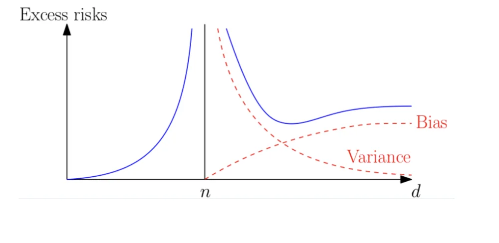
The formulas of both regimes in one picture. The variance explodes at d = n and falls on both sides. Far to the right the risk goes to 0 only if there is no signal to lose.

B. Where is the threshold?

Model	Threshold
linear model or random features with $m$ features	$m=n$
polynomial of degree $p$	$p+1=n$
network with $K$ outputs	number of parameters $=n\cdot K$

C. Minimum norm solution and gradient descent

1. $X{X}^{\top }$: the $n\times n$ matrix of scalar products of the data points.
2. Invert it. For $2\times 2$: ${\left(\begin{array}{cc}a& b\\ c& d\end{array}\right)}^{-1}=\frac{1}{ad-bc}\left(\begin{array}{cc}d& -b\\ -c& a\end{array}\right)$.
3. $\alpha =(X{X}^{\top }{)}^{-1}y$ and $w^{\star }=X^{\top }\alpha ={\sum }_i{\alpha }_i{x}_i$.
4. Checks: $X{w}^{\star }=y$. Any other solution minus $w^{\star }$ lies in $\ker X$ and has a larger norm.

You see	It means
gradient descent from $w_0=0$	converges to $w^{\star }$, the minimum norm solution
gradient descent from $w_0\ne 0$	converges to $w^{\star }$ plus the kernel part of $w_0$: the solution closest to the start
one step	$w_{t+1}=w_t-\eta X^{\top }(X{w}_t-y)$
allowed step size	$\eta <2/{\lambda }_{\max }(X{X}^{\top })$
logistic loss on separable data	the norm diverges, the direction converges to the maximum margin separator

D. Risk formulas for isotropic Gaussian inputs

Regime	Variance	Bias
under-parameterized, $n>d+1$ (OLS)	$\frac{{\sigma }^{2}d}{n-d-1}$	0
over-parameterized, $d>n+1$ (minimum norm)	$\frac{{\sigma }^{2}n}{d-n-1}$	$\Vert {\theta }^{\ast }{\Vert }^2\frac{d-n}{d}$

• ${\theta }^{\ast }=0$: only the variance, it goes to 0 for $d\gg n$. Benign.
• ${\theta }^{\ast }\ne 0$: for $d\gg n$ the bias approaches $\Vert {\theta }^{\ast }{\Vert }^2$, the risk of predicting 0. Not benign.
• Backwards: variance at most $q{\sigma }^2$ needs $d\ge n(1+\frac{1}{q})+1$, linear in $n$.

E. Spikes

• $P(\text{test point in a spike})\le 2n\exp (-cd{t}^2)$.
• At most $\delta$ needs $d\ge \frac{\ln (2n/\delta )}{c{t}^2}$, which grows only with $\ln n$.
• The spikes are harmless long before the variance is small. The variance condition $d\gg n$ is the binding one.

F. General covariance

Variance term ${\sigma }^2(\frac{k}{n}+n\frac{{\sum }_{i>k}{\lambda }_i^2}{({\sum }_{i>k}{\lambda }_i{)}^2})$, bias term ${\sum }_i{\lambda }_i{\theta }_i^{\ast 2}(\frac{r}{{\lambda }_i+r}{)}^2$ with $r=\frac{1}{n}{\sum }_{j>k}{\lambda }_j$.

You see	It means
a flat tail of $L$ equal eigenvalues	tail part of the variance $=n/L$: small for a long tail
one dominant tail eigenvalue	tail part $=n$: the variance does not vanish
signal on a large eigenvalue, ${\lambda }_i\gg r$	the factor $(\frac{r}{{\lambda }_i+r}{)}^2$ is tiny: almost nothing is lost
signal on a tail direction, ${\lambda }_i\ll r$	the factor is close to 1: the signal is lost
few large eigenvalues, then many tiny ones, signal on the large ones	benign overfitting
few large, then only few small ones	interpolates, but the variance stays large
many large eigenvalues	the bias stays high (the isotropic case)

G. Traps

• Minimum norm uses $X{X}^{\top }$ ($n\times n$), not $X^{\top }X$.
• Only the start at 0 gives the minimum norm solution.
• Interpolation alone is not benign. Compare the risk with the predictor 0.
• Under-parameterized has $n-d-1$ in the denominator, over-parameterized $d-n-1$.
• The spike condition is logarithmic in $n$, the variance condition linear.

References

All sources cited on the slides, in slide order (33 entries)

Slide	Source	Key point
9	Zhang, Bengio, Hardt, Recht and Vinyals (cited as Bengio et al.), “Understanding deep learning requires rethinking generalization”, 2017	networks fit random labels
13	Belkin, Hsu, Ma and Mandal, “Reconciling modern machine-learning practice and the classical bias-variance trade-off”, PNAS 2019	double descent
13, 134	Belkin, “Fit without fear: remarkable mathematical phenomena of deep learning through the prism of interpolation”, Acta Numerica 2021	interpolation, loss landscape
13, 49, 64, 86	Bartlett, Montanari and Rakhlin, “Deep learning: a statistical viewpoint”, Acta Numerica 2021	benign overfitting, aligned covariance
18, 34, 43, 64, 142	Bach, Learning Theory from First Principles, Fig. 12.3, Sec. 12.1.1, 12.1.2, 12.2.3, 12.3	random features, implicit bias, gradient flow
25	Hardt and Recht, Patterns, Predictions, and Actions	single descent figure
26, 28	Curth, Jeffares and van der Schaar, “A U-turn on double descent”, NeurIPS 2023	counting parameters
27	Meng et al., “Multiple descent in the multiple random feature model”, JMLR 2024	triple descent
44	Soudry, Hoffer, Nacson, Gunasekar and Srebro, “The implicit bias of gradient descent on separable data”, JMLR 2018	max-margin direction
47, 140	Jacot, Gabriel and Hongler, “Neural tangent kernel: convergence and generalization in neural networks”, NeurIPS 2018	NTK
47, 140	Arora, Du, Hu, Li, Salakhutdinov and Wang, “On exact computation with an infinitely wide neural net”, NeurIPS 2019	gradient flow, NTK
47	Gunasekar et al., 2018	deep linear networks, max margin
47	Lyu and Li, 2019	homogeneous networks, margin
47	Gunasekar et al., 2017	matrix factorization, low rank
48	Blanc et al., 2020	implicit bias of SGD noise
48	Damian et al., 2021	implicit bias of SGD noise
49, 64	Bartlett, Long, Lugosi and Tsigler, “Benign overfitting in linear regression”, PNAS 2020	benign overfitting
49	Tsigler and Bartlett, “Benign overfitting in ridge regression”, JMLR 24(123), 2023	ridge
49, 57	Hastie, Montanari, Rosset and Tibshirani, “Surprises in high-dimensional ridgeless least squares interpolation”, Annals of Statistics 2022	Theorem 3 (benign overfitting in the toy setup)
103, 105	Zhou, Sutherland and Srebro, “On uniform convergence and low-norm interpolation learning”, NeurIPS 2020	uniform convergence
105	Shamir, “The implicit bias of benign overfitting”, 2022	benign overfitting
112	Pinkus, “Approximation theory of the MLP model in neural networks”, Acta Numerica 1999	universal approximation
118	Telgarsky, “Benefits of depth in neural networks”, COLT 2016	depth vs. width
121	Shamir, “Distribution-specific hardness of learning neural networks”, JMLR 19(32), 2018	Theorem 7 (hardness of learning a small network)
123	Bubeck and Selke, “A universal law of robustness via isoperimetry”, NeurIPS 2021 / J. ACM 2023	robust interpolation
135	Cooper, “The loss landscape of overparameterized neural networks”, arXiv 2018	manifold of minima
135	Simsek et al., “Geometry of the loss landscape in overparameterized neural networks: symmetries and invariances”, ICML 2021	connected minima
136	Frankle et al., “Linear mode connectivity and the lottery ticket hypothesis”, ICML 2020	low-loss paths
137	Li, Tang and Sun, “On the benefit of width for neural networks”, SIAM J. Optimization 2022	no bad basins
137	Li, Ding and Sun, “Over-parameterized deep neural networks have no strict local minima for any continuous activations”	no strict local minima
138	Cohen, Damian, Talwalkar, Kolter and Lee, “Understanding optimization in deep learning with central flows”, ICLR 2025 (blog)	edge of stability
139	Li et al., “Visualizing the loss landscape of neural nets”, NeurIPS 2018	skip connections
140	Chizat, Oyallon and Bach, “On lazy training in differentiable programming”, NeurIPS 2019	lazy regime

Related

• Previous: Lecture 7: Data, Measurement and Validity · Next: Lecture 9.1: Fairness · Course: Overview · Formula Sheet · Glossary
• Concepts: Double Descent, Implicit Regularization, Benign Overfitting, Universal Approximation, Neural Tangent Kernel, Random Features, Bias-Variance Decomposition
• Exercises: Sheet 6, Exercise 2 (linear regression in different regimes); Sheet 9, Exercise 1 (the second descent for random features); Sheet 10, Exercise 1 (loss curves and the four regimes)