Lecture 6: Aggregation, Bagging and Boosting

TL;DR

1. Ensembles: there is no single best classifier (No Free Lunch), so combine many classifiers into one “committee”. Two opposing principles: random forests average many deep, overfitting trees (reduce variance); boosting combines many underfitting weak learners with specific weights (reduce bias).
2. Bootstrap approximates the distribution of an estimate by recomputing it on $B$ resamples. Bagging averages the $B$ bootstrap estimates: with pairwise correlation $\rho$ the variance is $\rho {\sigma }^2+(1-\rho )\frac{{\sigma }^2}{B}$ instead of ${\sigma }^2$, so success depends on how independent the estimates are.
3. Random forests: bagged spatial decision trees, each grown on a random subsample with the split dimension chosen from a random subset of $m\approx d/3$ dimensions. A forest can be consistent even if its individual (deep) trees are not.
4. AdaBoost: start with uniform weights; in round $t$ fit a weak learner $h_t$ with weighted error ${\epsilon }_t$, give it the vote $w_t=\frac{1}{2}\log (\frac{1}{{\epsilon }_t}-1)$, multiply the weights by $e^{-w_t{y}_i{h}_t(x_i)}$ and renormalize. Output $\mathrm{sign}({\sum }_t{w}_t{h}_t(x))$.
5. Theorem 1 (training error of AdaBoost): if every ${\epsilon }_t\le \frac{1}{2}-\gamma$, the training error is at most $\exp (-2{\gamma }^{2}T)$. Proof: $1\{\text{error}\}\le e^{-yf(x)}$, telescoping $Z_T={\prod }_t{Z}_{t+1}/Z_t$ with $Z_{t+1}/Z_t=2\sqrt{{\epsilon }_{t+1}(1-{\epsilon }_{t+1})}\le e^{-2{\gamma }^2}$.
6. Test error: VC bound with $\mathrm{VC}({\mathcal{H}}_T)\lesssim T\cdot \mathrm{VC}(\mathcal{B})\log (T\mathrm{VC}(\mathcal{B}))$ (needs $T/n\to 0$); the margin bound does not depend on $T$ and explains why boosting keeps improving after zero training error. Weak and strong PAC learnability are equivalent. Gradient boosting fits each new base learner to the negative gradient of the loss; AdaBoost is the special case of the exponential loss.

Exam relevance

• Real exam, task type “AdaBoost” (4 P): all formulas are given, a toy data set with a plot; compute $h_1$, ${\epsilon }_1$, $w_1$, the new weights $D^{(2)}$ (with normalization) and $h_2$, then comment on the behaviour, for example whether stumps can solve an XOR configuration or what happens when ${\epsilon }_t=\frac{1}{2}$. Train it with the task and the widget below.
• Real exam, multiple choice: bagging came up (what it reduces, when it works).
• Mock exam, task 7: prove that the training error is at most $Z_T$ and derive $\exp (-2{\gamma }^{2}T)$ from $Z_t/Z_{t-1}=2\sqrt{{\epsilon }_t(1-{\epsilon }_t)}$. The full proof is below.
• Sheet 7, Exercise 3 (why bagging reduces variance); Sheet 8 (boosting stumps by hand, implementing AdaBoost, gradient boosting and the choice of the base learner).
• Everything in one go: the cheat sheet with two full integration tasks at the end of this note.

Exam essentials (8 cards)

Only what you should know by heart in the exam. Click a card for the answer, or press a to go through them as flashcards. For Anki: deck of this lecture.

Variance of the average of $B$ bagged estimates?

Answer

Variance ${\sigma }^2$ each, pairwise correlation $\rho$: $\rho {\sigma }^2+(1-\rho )\frac{{\sigma }^2}{B}$.
The shared part $\rho {\sigma }^2$ stays, only the rest averages out.

Random forests vs. boosting: which error does each reduce?

Answer

Random forests average many deep, overfitting trees: they reduce variance.
Boosting combines many underfitting weak learners with weights: it reduces bias.

How many of the original points does a bootstrap sample contain?

Answer

About 63% of the distinct points, since $(1-\frac{1}{n}{)}^n\to e^{-1}\approx 0.37$ are never drawn.

AdaBoost: weighted error and vote of the weak learner $h_t$?

Answer

${\epsilon }_t={\sum }_i{D}_{i}1[h_t(x_i)\ne y_i]$
$w_t=\frac{1}{2}\log (\frac{1}{{\epsilon }_t}-1)=\frac{1}{2}\ln \frac{1-{\epsilon }_t}{{\epsilon }_t}$ (also written ${\alpha }_t$)

AdaBoost: weight update and final classifier?

Answer

$D_i\leftarrow D_i{e}^{-w_t{y}_i{h}_t(x_i)}/Z$. After the update the misclassified points carry exactly half of the weight.
Output: $\mathrm{sign}({\sum }_t{w}_t{h}_t(x))$.

Training error bound of AdaBoost?

Answer

If every ${\epsilon }_t\le \frac{1}{2}-\gamma$: training error $\le {\prod }_{t}2\sqrt{{\epsilon }_t(1-{\epsilon }_t)}\le e^{-2{\gamma }^{2}T}$.

Can AdaBoost with decision stumps fit XOR?

Answer

No. A weighted sum of stumps is additive in the coordinates, and XOR needs an interaction of both.

How is AdaBoost related to gradient boosting?

Answer

Gradient boosting fits each new base learner to the negative gradient of the loss.
AdaBoost is the special case of the exponential loss $e^{-yf(x)}$.

Overview: 1. Ensembles, bootstrap and bagging, 2. Random forests, 3. Boosting: weak and strong learners, 4. AdaBoost and its training error, 5. The test error of AdaBoost, 6. Gradient boosting.

Motivation from statistics: ensembles, bagging, bootstrap

Combining classifiers in ensembles

Slides 3-5

(Literature: the statistics point of view is discussed extensively in Hastie, Tibshirani and Friedman.)

• No Free Lunch: there is no single best classifier, so we need to select classifiers, ideally based on their inductive bias.
• Empirically, many classifiers are specialized: very good (or very confident) in some part of the space and poor in others.
• Idea: combine many classifiers into one big, overarching “committee” classifier that is confident and good in all parts of the space. There are many approaches; the keyword is ensemble methods. Many of them originate in statistics.

Bootstrap

Slides 6-9

Cross validation estimates the test error by training on random subsets and testing on others, repeating the procedure and averaging the results. Statistics has a whole family of methods following this principle: the bootstrap.

The bootstrap method

We want to estimate a parameter $\Theta$ of an unknown distribution (for example the test error of a classifier) and have a sample $X_1,\dots ,X_n$ and an estimate $\hat{\Theta }$. To judge the estimate we would like to know its distribution (its variance, confidence sets), but the distribution is unknown.

Idea: construct an empirical distribution of the estimate. Draw a subsample of $m$ points from the original sample (with or without replacement), compute the estimate on it, and repeat $B$ times. The bootstrap estimates ${\hat{\Theta }}_1,\dots ,{\hat{\Theta }}_B$ form an empirical distribution that approximates the distribution of $\hat{\Theta }$: use it for the mean, the variance, confidence sets.

Why and when does it make sense?

• If the ${\hat{\Theta }}_b$ were independent, the Glivenko-Cantelli theorem would say their empirical distribution approximates the true one.
• But they are not independent: they are computed on largely overlapping samples. The question of bootstrap theory is under which conditions the empirical distribution is still a good approximation.
• Intuitively this works if random reweighting of the observed data mimics real sampling variability. It tends to work for statistics based on averaging (mean, variance), and tends not to for extreme value statistics (maximum or minimum of a distribution).

Standard textbooks: Efron and Tibshirani, An Introduction to the Bootstrap; Shao and Tu, The Jackknife and Bootstrap (more mathematical).

Mini example (not on the slides): how many points does a bootstrap sample miss?

Drawing $n$ points with replacement from $n$, a fixed point is never drawn with probability $(1-\frac{1}{n}{)}^n\to e^{-1}\approx 0.368$. So each bootstrap sample contains only about 63% of the distinct original points; the rest can serve as “out-of-bag” test points.

Bagging to reduce the variance

Slides 10-11

Bagging (bootstrap aggregation)

Generate $B$ bootstrap samples, compute the estimate ${\hat{\Theta }}_1,\dots ,{\hat{\Theta }}_B$ on each, and take the average as the final estimate:

$${\hat{\Theta }}_{bag}=\mathrm{mean}({\hat{\Theta }}_1,\dots ,{\hat{\Theta }}_B)$$

The hope is that ${\hat{\Theta }}_{bag}$ has a much smaller variance than each individual ${\hat{\Theta }}_b$.

Variance of the bagged estimate

If the ${\hat{\Theta }}_b$ are identically distributed with variance ${\sigma }^2$:

• i.i.d.: $\mathrm{Var}({\hat{\Theta }}_{bag})={\sigma }^2/B$, a reduction by the factor $B$;
• pairwise correlation $\rho >0$:

$$\mathrm{Var}({\hat{\Theta }}_{bag})=\rho {\sigma }^2+(1-\rho )\frac{{\sigma }^2}{B}$$

For small $\rho$ and large $B$ this is still good. Whether bagging succeeds depends on how independent we manage the ${\hat{\Theta }}_b$ to be.

Derivation of the correlated case

$\mathrm{Var}\left(\frac{1}{B}{\sum }_b{\hat{\Theta }}_b\right)=\frac{1}{B^2}({\sum }_b\mathrm{Var}({\hat{\Theta }}_b)+{\sum }_{b\ne b^{\prime }}\mathrm{Cov}({\hat{\Theta }}_b,{\hat{\Theta }}_{b^{\prime }}))=\frac{1}{B^2}(B{\sigma }^2+B(B-1)\rho {\sigma }^2)=\rho {\sigma }^2+\frac{(1-\rho ){\sigma }^2}{B}$. $\square$

Trap

Bagging reduces variance, not bias: averaging many estimates with the same systematic error keeps that error. For $B\to \infty$ the variance does not go to 0 but to $\rho {\sigma }^2$.

Memory aid

The shared part stays, the private part averages out: $\rho {\sigma }^2+(1-\rho ){\sigma }^2/B$.

Task: the variance of bagging

Exam-style task: bagging (4 P)

Math: variance of an average

Each tree of an ensemble predicts at a fixed test point with variance ${\sigma }^2=4$ and bias $0.5$; any two trees have correlation $\rho =0.2$.

(a) (1 P, easy) Compute the variance of the average of $B=10$ trees and of $B\to \infty$ trees.

(b) (1.5 P, harder) How many trees are needed so that the variance is within 10% of its limit? What is the expected squared error of the infinite ensemble at this point (squared bias plus variance)?

(c) (1.5 P, transfer) A random forest decorrelates the trees by choosing each split among a random subset of dimensions, which lowers $\rho$ to $0.05$ but raises ${\sigma }^2$ to $5$. Is this a good trade for a large forest? What does bagging do to the bias?

Solution

(a) $B=10$: $0.2\cdot 4+0.8\cdot 4/10=0.8+0.32=1.12$. $B\to \infty$: $\rho {\sigma }^2=0.8$. (1 P)

(b) Need $(1-\rho ){\sigma }^2/B\le 0.08$: $3.2/B\le 0.08⟺B\ge 40$. Error of the infinite ensemble: $0.5^2+0.8=1.05$ (a single tree: $0.25+4=4.25$). (1.5 P)

(c) Limit variance $0.05\cdot 5=0.25<0.8$: yes, for large $B$ the lower correlation wins (with $B=1$ it would be worse, $5>4$). The bias stays $0.5$: averaging does not change the bias. (1.5 P)

Two opposing principles: bagging vs. boosting

Slide 12

• Random forests: start with an ensemble of many deep decision trees that completely overfit, then build a naive average over many such trees and obtain a prediction function that generalizes well.
• Boosting: use an ensemble of super-simple classifiers (decision stumps: trees of depth 1 or 2) that completely underfit, then build a specifically weighted average and obtain a prediction function that generalizes well.

Currently, random forests and boosting are about the most successful algorithms for machine learning on tabular data.

Random forests

Bagging decision trees

Slides 13-15

(Literature: Breiman, “Random forests”, Machine Learning 2001; overview: Biau and Scornet, “A random forest guided tour”, Test 2016; Hastie, Tibshirani and Friedman Ch. 8, 9, 15; Shalev-Shwartz and Ben-David Ch. 18; Tang, Garreau and von Luxburg, “When do random forests fail?”, NeurIPS 2018; Haghiri, Garreau and von Luxburg, “Comparison-based random forests”, ICML 2018.)

Apply bagging to regression or classification: repeatedly take a subsample, train a baseline algorithm on it to get $f_1,\dots ,f_B$, and for a test point average the outputs, $y_{bag}=\mathrm{mean}(f_1(x),\dots ,f_B(x))$.

Choosing the baseline algorithm:

• The procedure is computationally expensive, so use a reasonably simple baseline.
• Bagging reduces the variance most if there is little correlation between the classifiers: this is what we need to achieve.
• If the classifiers have a strong bias, bagging cannot do anything about it.

A standard choice is decision trees, aggregated to a “forest”.

Spatial decision trees

Slides 16-19

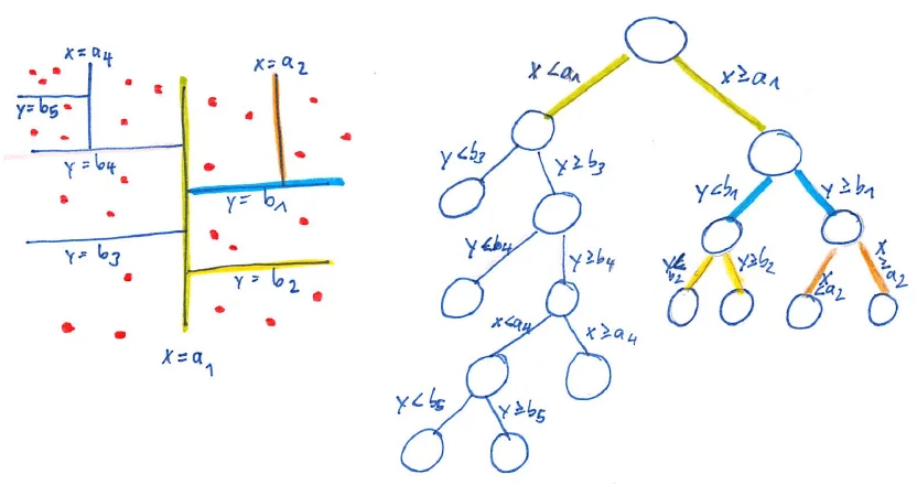
Slide 16: a spatial partition tree on ℝᵈ. Left the partition of the space, right the tree.

Spatial decision tree (high-level)

• Construct the tree recursively: for each cell, consider various splits in different dimensions and select one; keep splitting until cells contain a predefined number of points.
• Split criterion (one example): split the points of a cell into $A$ and $A^c$, predict the means ${\hat{Y}}_A$ and ${\hat{Y}}_{A^c}$ and compute

$$erro{r}_{split}=\sum _{i\in A}({\hat{Y}}_A-Y_i{)}^2+\sum _{i\in A^c}({\hat{Y}}_{A^c}-Y_i{)}^2$$

• Typically axis-parallel splits: for every dimension $k=1,\dots ,d$ find the best splitting point $s_k$ (greedily) with error $erro{r}_{split,k}$; use the dimension with the smallest error.
• Prediction: find the cell of the test point and predict the average of the training labels in the cell (regression) or the majority vote (classification).

Depth of the tree / leaf size. Keep splitting until a cell has fewer than $n_{leaf}$ points.

• For a consistent single tree, the number of points per leaf has to increase slowly with $n$, for example $n_{leaf}=\log n$: shallow trees.
• Random forests often use deep trees with a constant number of points per leaf (in the extreme $n_{leaf}=1$). A single such tree would be a disaster (overfitting), but a forest of them can be consistent.

The random forest algorithm

Slides 20-22

Random forest

A random forest uses bagging to combine many spatial decision trees. Each tree is constructed randomly: on a random sample of the input points, and each split chooses the splitting dimension among a random subset of the dimensions.

Input: data points in ℝ^p. Parameters: B, N, n_min, m.
1. For b = 1 to B:
   (a) Draw a bootstrap sample Z* of size N from the training data.
   (b) Grow a random-forest tree T_b on Z* by recursively repeating, for each
       terminal node, until the minimum node size n_min is reached:
       i.   select m variables at random from the p variables,
       ii.  pick the best variable / split point among the m,
       iii. split the node into two daughter nodes.
2. Output the ensemble {T_b}, b = 1..B.
Regression: f(x) = (1/B) Σ_b T_b(x).  Classification: majority vote of the T_b(x).

(Algorithm 15.1 of Hastie, Tibshirani and Friedman.)

Parameters:

• the subsample size: reasonably large, with or without replacement (without replacement one often takes the size of the original sample);
• the number $m$ of dimensions from which the best one is picked: typically around $d/3$;
• the number $B$ of trees: large;
• the leaf size $n_{min}$: deep trees ($n_{min}=1$, then $B$ must be large) or shallow trees ($n\approx \log n$).

In principle the algorithm is not extremely sensitive to many of the parameters, but in a completely bad regime the trees can under- or overfit (Biau’s guided tour; “When do random forests fail?”).

Consistency of random forests

Slides 23-26

Consistency

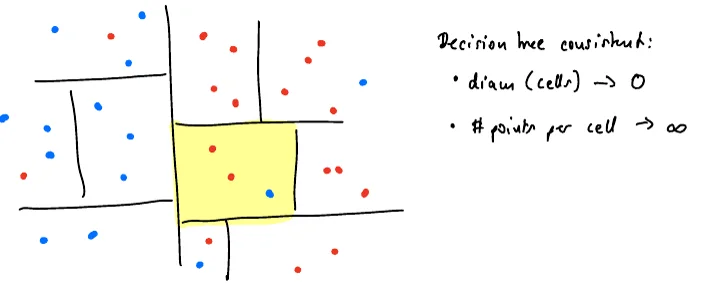
• A single spatial decision tree is consistent if the diameter of all cells converges to 0 and at the same time the number of points per cell tends to infinity as $n\to \infty$ (can you prove it?).
• If all individual trees are consistent, so is the random forest (Biau, “Analysis of a random forests model”, JMLR 2012).
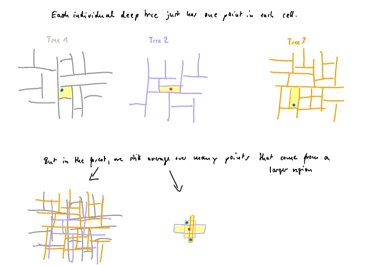
• Curiously, a random forest can be consistent even if all its individual trees are not, in particular for deep trees (Scornet, “On the asymptotics of random forests”, Journal of Multivariate Analysis 2016). This is not obvious and depends on the exact setup (“When do random forests fail”, Tang, Garreau and von Luxburg 2018).

Slide 23: consistency of a single tree: diam(cell) → 0 and #points per cell → ∞.

Slide 25: each deep tree has one point per cell, but the forest averages over many points that come from a larger region.

Outlook: comparison-based random forests. Random forests need a Euclidean representation. Alternative, the comparison tree: in the current cell pick two random points $x_1,x_2$, and split according to whether each point is closer to $x_1$ or to $x_2$. This can also lead to consistent classification and regression (Haghiri, Garreau and von Luxburg 2018) and works really well empirically.

Slide 26: splits of a comparison-based tree.

Boosting

Strong and weak learners

Slides 27-30

(Literature: Shalev-Shwartz and Ben-David Sec. 10; Hastie, Tibshirani and Friedman (a long chapter on boosting and gradient boosting); Schapire and Freund, Boosting: Foundations and Algorithms (a whole, very readable book); original paper Schapire and Freund 1995.)

Strong and weak learners, intuitively

A strong learner approximates the true solution up to a small error $\epsilon$; constructing strong learners is the goal of machine learning, but they are often hard to construct and computationally expensive. A weak learner is just slightly better than random guessing: for balanced classes its 0-1 loss is $0.5-\epsilon$ (its accuracy $0.5+\epsilon$).

The idea of boosting is to combine many weak learners to obtain a strong learner.

Weak and strong PAC learners (formally)

Data space $\mathcal{X}$ with distribution $\mathcal{D}$, hypothesis class $\mathcal{H}$, and the true classifier lives in it: $y=h(x)$ for a deterministic $h\in \mathcal{H}$ (PAC = probably approximately correct).

• $\mathcal{H}$ is strongly PAC-learnable if there is an algorithm such that for every $\epsilon ,\delta >0$, every $\mathcal{D}$ and every $h\in \mathcal{H}$, run on $n(\delta ,\epsilon )$ training points, it returns $\hat{h}$ with 0-1 loss at most $\epsilon$ with probability at least $1-\delta$.
• $\mathcal{H}$ is weakly PAC-learnable if for some $\gamma >0$ there is an algorithm that takes $n(\delta )$ examples and returns $\hat{h}$ with ${\ell }_{01}(\hat{h})\le \frac{1}{2}-\gamma$ with probability at least $1-\delta$.
• Efficiently weak / strong PAC-learnable: the algorithm runs in polynomial time (in particular sees only polynomially many samples).

For some time researchers wondered whether weak learnability is “easier” than strong learnability; see the end of this lecture.

Boosting: the outline and a toy example

Slides 31-36

Boosting, the outline

• Given $n$ training points, the algorithm proceeds in $T$ rounds.
• Training points have weights $w_i$ that change from round to round and always add up to 1.
• In each round, train the weak classifier on the weighted points, then update the weights: increase the weight of misclassified points, decrease the weight of correctly classified points.
• The final classifier is a weighted sum of the weak classifiers of all rounds.

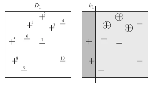
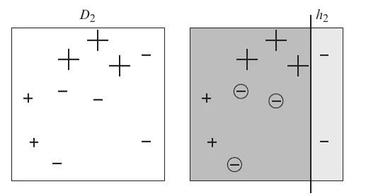
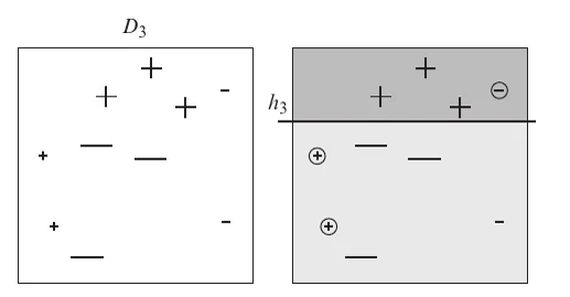
Slide 32: uniform weights D₁ and the weak classifier h₁ (circled: its mistakes).

Slide 33: new weights D₂ (symbol size) and h₂, which gets the heavy points right.

Slide 34: weights D₃ and the third weak classifier h₃.

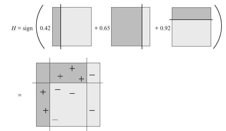
Slide 35: the combination H = sign(0.42·h₁ + 0.65·h₂ + 0.92·h₃), a weighted majority vote (figures from the Schapire/Freund book).

First remarks (slide 36):

• Unlike random forests (randomness through subsampling points and dimensions), the training set in boosting is always the same; only the weights change.
• By reweighting, the algorithm focuses on examples it finds difficult or on aspects overlooked so far.
• Once a point has accumulated weight larger than 0.5, the weak learner will get it right. But it is not obvious that this helps the final classifier, because there are many points to get right. The question is how to combine the evidence of the weak classifiers into a strong classifier.

The AdaBoost algorithm

Slides 37-39

AdaBoost (slide 38, from Understanding Machine Learning)

Input: training set $S=(x_1,y_1),\dots ,(x_m,y_m)$ with $y_i\in \{\pm 1\}$, weak learner WL, number of rounds $T$.

Initialize the sample weights $D^{(1)}=(\frac{1}{m},\dots ,\frac{1}{m})$.

For $t=1,\dots ,T$:

• invoke the weak learner $h_t=\mathrm{WL}(D^{(t)},S)$;
• compute the error at step $t$: ${\epsilon }_t=\sum _{i=1}^m{D}_i^{(t)}1[y_i\ne h_t(x_i)]$;
• let the update factor $w_t=\frac{1}{2}\log (\frac{1}{{\epsilon }_t}-1)$;
• update $D_i^{(t+1)}=\frac{D_i^{(t)}\exp (-w_t{y}_i{h}_t(x_i))}{{\sum }_{j=1}^m{D}_j^{(t)}\exp (-w_t{y}_j{h}_t(x_j))}$ for all $i$.

Output the hypothesis $h_s(x)=\mathrm{sign}(\sum _{t=1}^T{w}_t{h}_t(x))$.

Why is it plausible that it works?

If the final classifier $h_s$ errs on a training point $x$, then (being a weighted majority vote) most weak classifiers got $x$ wrong. So the weight of $x$ was increased very often and must still be large after the final round. But only few points can have large weights, because all weights add up to 1. So only few points can be misclassified by the final classifier.

Computing the update by hand

Since $y_i{h}_t(x_i)=+1$ for correct and $-1$ for wrong points, and $e^{w_t}=\sqrt{(1-{\epsilon }_t)/{\epsilon }_t}$:

• correct points are multiplied by $e^{-w_t}$, wrong points by $e^{w_t}$;
• after normalizing, the misclassified points together have weight exactly $\frac{1}{2}$: each wrong point gets $D_i^{(t)}/(2{\epsilon }_t)$, each correct point $D_i^{(t)}/(2(1-{\epsilon }_t))$.

Consequence: the old $h_t$ has weighted error exactly $\frac{1}{2}$ under $D^{(t+1)}$, so the next weak learner has to do something different.

Special cases of ${\epsilon }_t$

• ${\epsilon }_t=\frac{1}{2}$: $w_t=\frac{1}{2}\log 1=0$. The weak learner is useless, the weights do not change, and AdaBoost makes no progress.
• ${\epsilon }_t>\frac{1}{2}$: $w_t<0$; the classifier is flipped (for stumps, the flipped stump is in the class anyway).
• ${\epsilon }_t=0$: $w_t=\infty$; one weak learner already classifies everything correctly.

AdaBoost with axis-parallel decision stumps. Point size is the current weight, the orange line the last stump and its circled mistakes, the shading the sign of f_T. The tables list εₜ, wₜ and all weights, like in the exam. The preset "Task" is the data of the task below, "XOR" shows the case εₜ = ½.

Memory aid

Better than a coin flip → positive vote $\alpha =\frac{1}{2}\ln \frac{1-\epsilon }{\epsilon }$. After the update the mistakes carry exactly half of the weight, so the next learner has to fix them.

Theorem 1: the training error bound

Slides 40-45

Theorem 1 (training error of AdaBoost)

Run AdaBoost on a training set of size $n$ for $T$ rounds, and assume that in each round $t$ the weak learner returns a function with weighted training 0-1 error ${\epsilon }_t\le \frac{1}{2}-\gamma$ for some $\gamma >0$. Then the training 0-1 error of the final output function is at most

$$\exp (-2{\gamma }^{2}T)$$

The training error decreases exponentially in the number of rounds.

Proof

Step 1: bound the 0-1 loss by the exponential loss. Let $f_t={\sum }_{p\le t}{w}_p{h}_p$ (with $f_0\equiv 0$) and

$$Z_t=\frac{1}{n}\sum _{i=1}^n\exp (-y_i{f}_t(x_i)),Z_0=1$$

the empirical exponential loss. A point is misclassified iff $y_i{f}_T(x_i)\le 0$, and $1\{z\le 0\}\le e^{-z}$. So

$$\text{training error}(f_T)=\frac{1}{n}\sum _{i}1\{\mathrm{sign}{f}_T(x_i)\ne y_i\}\le \frac{1}{n}\sum _i{e}^{-y_i{f}_T(x_i)}=Z_T$$

(For $\pm 1$-valued $h$: $1(h(x)\ne y)$ is 0 or 1, while $e^{-yh(x)}$ is $1/e\approx 0.37$ or $e\approx 2.7$.)

Step 2: telescoping. Since $Z_0=1$,

$$Z_T=\frac{Z_T}{Z_{T-1}}\cdot \frac{Z_{T-1}}{Z_{T-2}}\cdots \frac{Z_1}{Z_0}$$

and it suffices to show $\frac{Z_{t+1}}{Z_t}\le \exp (-2{\gamma }^2)$ for every factor.

Step 3: each factor. By induction, $D_i^{(t+1)}=\frac{\exp (-y_i{f}_t(x_i))}{{\sum }_j\exp (-y_j{f}_t(x_j))}$. Since $f_{t+1}=f_t+w_{t+1}{h}_{t+1}$,

$$\frac{Z_{t+1}}{Z_t}=\frac{{\sum }_i{e}^{-y_i{f}_t(x_i)}{e}^{-y_i{w}_{t+1}{h}_{t+1}(x_i)}}{{\sum }_j{e}^{-y_j{f}_t(x_j)}}=\sum _i{D}_i^{(t+1)}{e}^{-y_i{w}_{t+1}{h}_{t+1}(x_i)}=(1-{\epsilon }_{t+1})e^{-w_{t+1}}+{\epsilon }_{t+1}{e}^{w_{t+1}}$$

With $e^{w_{t+1}}=\sqrt{(1-{\epsilon }_{t+1})/{\epsilon }_{t+1}}$ both terms equal $\sqrt{{\epsilon }_{t+1}(1-{\epsilon }_{t+1})}$:

$$\frac{Z_{t+1}}{Z_t}=2\sqrt{{\epsilon }_{t+1}(1-{\epsilon }_{t+1})}$$

With ${\epsilon }_{t+1}=\frac{1}{2}-{\gamma }_{t+1}$, ${\gamma }_{t+1}\ge \gamma$: $2\sqrt{\epsilon (1-\epsilon )}=\sqrt{1-4{\gamma }_{t+1}^2}\le \sqrt{1-4{\gamma }^2}$, and $1-\alpha \le e^{-\alpha }$ gives $\sqrt{1-4{\gamma }^2}\le e^{-2{\gamma }^2}$.

Step 4: combine. $\text{training error}(f_T)\le Z_T={\prod }_{t=0}^{T-1}\frac{Z_{t+1}}{Z_t}\le (\exp (-2{\gamma }^2){)}^T=\exp (-2{\gamma }^{2}T)$. $\square$

(Details: Shalev-Shwartz and Ben-David Sec. 10, Schapire and Freund Sec. 3.1.)

Why $w_t=\frac{1}{2}\log (\frac{1}{{\epsilon }_t}-1)$?

The factor $(1-\epsilon )e^{-w}+\epsilon e^w$ is minimized exactly at $e^{2w}=(1-\epsilon )/\epsilon$: AdaBoost chooses the vote that decreases the exponential loss $Z_t$ as much as possible in each round.

Memory aid

Each round multiplies the bound by at most $e^{-2{\gamma }^2}$: the edge $\gamma$ over a coin flip counts squared, so a weak learner with $\epsilon =0.4$ needs about 350 rounds for $10^{-3}$.

Task: AdaBoost by hand

Exam-style task: AdaBoost with decision stumps (4 P)

Math: logs and exponentials

Five points on the real line: $x_i=i$ for $i=1,\dots ,5$ with labels $y=(+1,+1,-1,-1,+1)$. The weak learners are decision stumps $h_{\theta ,s}(x)=s$ if $x>\theta$ and $-s$ otherwise, with $s\in \{\pm 1\}$ and thresholds $\theta \in \{1.5,2.5,3.5,4.5\}$ (no constant classifiers). In each round the weak learner returns the stump with the smallest weighted error. Use the formulas of the AdaBoost algorithm.

(a) (1 P, easy) Determine $h_1$, ${\epsilon }_1$ and $w_1$.

(b) (1.5 P, harder) Compute $D^{(2)}$ (normalized) and determine $h_2$, ${\epsilon }_2$ and $w_2$.

(c) (1.5 P, transfer) Give the combined classifier $\mathrm{sign}(w_1{h}_1+w_2{h}_2)$ on the five points and its training error, and compare with the bound $Z_2={\prod }_{t}2\sqrt{{\epsilon }_t(1-{\epsilon }_t)}$. Then consider the XOR configuration $(0,0),(1,1)$ with label $+1$ and $(1,0),(0,1)$ with label $-1$ and stumps on either coordinate: what happens in the first round, and why?

Solution

(a) With uniform weights $\frac{1}{5}$, the stump ”$+1$ for $x<2.5$, $-1$ for $x>2.5$” ($\theta =2.5$, $s=-1$) only misclassifies $x=5$; every other stump makes at least two mistakes. ${\epsilon }_1=\frac{1}{5}$, $w_1=\frac{1}{2}\log (5-1)=\frac{1}{2}\log 4=\log 2\approx 0.693$. (1 P)

(b) Wrong point $x=5$: $\frac{1}{5}\cdot e^{\log 2}=\frac{2}{5}$; correct points: $\frac{1}{5}\cdot e^{-\log 2}=\frac{1}{10}$. Sum $=4\cdot \frac{1}{10}+\frac{2}{5}=\frac{4}{5}$. So $D^{(2)}=(\frac{1}{8},\frac{1}{8},\frac{1}{8},\frac{1}{8},\frac{1}{2})$ (the mistake now carries half the weight) (0.5 P). Weighted errors of the stumps that get $x=5$ right ($+1$ at $x=5$): $\theta =4.5,s=+1$ errs on $x=1,2$: $\frac{1}{4}$; $\theta =3.5,s=+1$ errs on $1,2,4$: $\frac{3}{8}$; $\theta =2.5,s=+1$ errs on $1,2,3,4$: $\frac{1}{2}$; $\theta =1.5,s=+1$ errs on $1,3,4$: $\frac{3}{8}$. Stumps with $-1$ at $x=5$ already pay $\frac{1}{2}$. So $h_2$: ”$+1$ for $x>4.5$”, ${\epsilon }_2=\frac{1}{4}$, $w_2=\frac{1}{2}\log 3\approx 0.549$. (1 P)

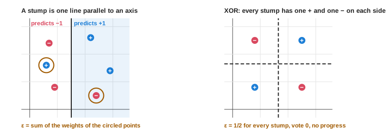
(c) $f_2=0.693h_1+0.549h_2$: at $x=1,2$: $0.693-0.549>0$, $+1$ ✓; at $x=3,4$: $-0.693-0.549<0$, $-1$ ✓; at $x=5$: $-0.693+0.549<0$, $-1$ ✗. Training error $\frac{1}{5}$. Bound: $2\sqrt{\frac{1}{5}\cdot \frac{4}{5}}\cdot 2\sqrt{\frac{1}{4}\cdot \frac{3}{4}}=0.8\cdot 0.866\approx 0.69\ge 0.2$ ✓ (0.75 P). XOR: every stump splits the square into two halves that each contain one $+$ and one $-$, so every stump has weighted error exactly $\frac{1}{2}$. Then $w_1=0$, the weights stay uniform and every later round finds the same situation: AdaBoost never makes progress. The weak learning assumption ${\epsilon }_t\le \frac{1}{2}-\gamma$ fails for stumps on XOR; one needs richer base learners (trees of depth 2). (0.75 P)

Task: how many rounds?

Exam-style task: the training error bound (4 P)

Math: solving e^(-cT) < δ

AdaBoost runs on $n=1000$ training points, and every weak learner has weighted error at most $0.4$.

(a) (1 P, easy) Give $\gamma$ and the bound of Theorem 1 (training error of AdaBoost) after $T=50$ rounds.

(b) (1.5 P, harder) After how many rounds is the training error guaranteed to be zero?

(c) (1.5 P, transfer) Using the sharper per-round factor $2\sqrt{\epsilon (1-\epsilon )}$ with $\epsilon =0.4$, how many rounds suffice? Why does zero training error not mean that you should stop?

Solution

(a) $\gamma =0.5-0.4=0.1$, bound $\exp (-2\cdot 0.01\cdot 50)=e^{-1}\approx 0.37$. (1 P)

(b) The training error is a multiple of $\frac{1}{n}$; if it is below $\frac{1}{n}$ it is 0. $e^{-2{\gamma }^{2}T}<\frac{1}{1000}⟺T>\frac{\ln 1000}{2{\gamma }^2}=\frac{6.91}{0.02}\approx 345.4$, so $T=346$ rounds. (1.5 P)

(c) $2\sqrt{0.4\cdot 0.6}\approx 0.980$, so we need $0.980^T<10^{-3}$: $T>\frac{\ln 1000}{-\ln 0.980}\approx \frac{6.91}{0.0204}\approx 339$ rounds. After zero training error the margins can still grow, and the margin bound (below) says the test error can keep decreasing; the VC bound, in contrast, gets worse with $T$. (1.5 P)

Bounding the test error of AdaBoost

A generalization bound based on VC theory

Slides 46-54

(Literature: Understanding Machine Learning.) Does the test error also improve during boosting? Yes, and there are many approaches to prove it; the lecture covers two.

The boosting class

If AdaBoost uses weak classifiers from a base class $\mathcal{B}$ (for example decision stumps), the final classifier lives in

$${\mathcal{H}}_T=\left\{\mathrm{sign}\right(\sum _{t=1}^T{w}_t{h}_t(x)\left)\right|w\in {\mathbb{R}}^T,h_t\in \mathcal{B}\}$$

Theorem 2 (VC dimension of the boosting class)

For a base class $\mathcal{B}$ and the corresponding boosting class ${\mathcal{H}}_T$, $T\in \mathbb{N}$:

$$\mathrm{VC}({\mathcal{H}}_T)\le T\cdot \mathrm{VC}(\mathcal{B})\log (T\cdot \mathrm{VC}(\mathcal{B}))$$

Proof sketch

Take a set $C=\{x_1,\dots ,x_n\}$ shattered by ${\mathcal{H}}_T$. A labeling of $C$ is produced by $f(x)={\sum }_t{w}_t{h}_t(x)$: first choose $h_1,\dots ,h_T\in \mathcal{B}$, then apply a linear classifier with weights $w$ to the vector $(h_1(x),\dots ,h_T(x))\in {\mathbb{R}}^T$. Count the labelings:

• Let $d=\mathrm{VC}(\mathcal{B})$. By Sauer-Shelah, the base class realizes at most $(en/d{)}^d$ labelings of $C$; choosing $T$ of them gives $(en/d{)}^{d\cdot T}$ possibilities.
• Linear classifiers on ${\mathbb{R}}^T$ have VC dimension about $T$ (Lecture 3), so they combine the base functions in at most $(en/T{)}^T$ ways.
• Together: about $(en/d{)}^{dT}\cdot (en/T{)}^T\le n^{(d+1)T}$ classifiers.

To shatter $C$ we need $2^n$ functions, which is possible as long as $2^n\le n^{(d+1)T}$. The $n$ where this stops to hold is the VC dimension; solving the equality gives $n\le 2\frac{(d+1)T}{\log 2}\log \frac{(d+1)T}{\log 2}$. Ignoring constants, this is the claim. $\square$

Final generalization bound

With the VC bound of Lecture 3 (constants ignored):

$$R(f_T)\le R_n(f_T)+\sqrt{\frac{d\log (n/d)-\log (\delta )}{n}},d=d_{\mathcal{H}}=T\cdot d_{\mathcal{B}}$$

The key quantity is $T{d}_{\mathcal{B}}/n$. The base class is simple (small constant $d_{\mathcal{B}}$), so we get generalization from training to test error if $T/n\to 0$.

Two ways to use it:

• train few rounds $T$, live with the training error reached so far, and conclude by VC arguments that the test error is of the same order;
• or train until the training error is really small and check how many rounds were needed: if $T$ is still small compared to $n$, the test error is small too; if $T$ is large compared to $n$, we have likely overfitted.

A generalization bound based on margins

Slides 55-57

The success of boosting is described even better by a margin-based theory. Normalize the non-negative weights of $f(x)={\sum }_{t=1}^T{w}_t{h}_t(x)$ such that ${\sum }_t{w}_t=1$. Then $yf(x)\in [-1,1]$ is the margin of the sample $(x,y)$: it says how close or how far the point is from being misclassified.

Margin bound (Schapire and Freund, Theorem 5.5)

Let the base classifiers have VC dimension $d$ and let $S$ be a sample of $m\ge d\ge 1$ i.i.d. examples. With probability at least $1-\delta$, every weighted average $f\in \mathrm{co}(\mathcal{H})$ (the convex hull of the base class; AdaBoost functions are contained in it) satisfies

$$\begin{array}{rl}{P}_{\mathcal{D}}(yf(x)\le 0)\le & P_S(yf(x)\le \theta )\\ & +O\left(\sqrt{\frac{d\log (m/d)\log (m{\theta }^2/d)}{m{\theta }^2}+\frac{\log (1/\delta )}{m}}\right)\end{array}$$

for all $\theta >\sqrt{8d\ln (em/d)/m}$. Somewhat simplified, ignoring constants: for all $\theta \ge \sqrt{d/m}$,

$$P_{true}(yf(x)\le 0)\le P_{empirical}(y_{i}f(x_i)\le \theta )+O\left(\frac{1}{\theta }\sqrt{\frac{d\log n}{n}}\right)$$

What the margin bound says

• Left side: the test error. First term on the right: not the training error, but the fraction of training points with margin at most $\theta$.
• If the margin is large, choose $\theta$ as a large constant: few points lie in the margin (small first term), and the complexity term is small too because $\theta$ is not close to 0.
• The complexity term contains the VC dimension of the base classifier, not of the final classifier: the number $T$ of rounds does not enter the bound.
• This matches the empirical observation that boosting often keeps improving after the training error is already 0: the margin $\theta$ can still increase, while increasing $T$ does not hurt.

Equivalence of weak and strong PAC learnability

Slides 58-59

Theorem 3 (weak = strong PAC learnability)

A hypothesis class $\mathcal{H}$ is (efficiently) weakly PAC-learnable if and only if it is (efficiently) strongly PAC-learnable.

Do you find it surprising? The proof (Schapire and Freund, Sec. 4.3) is not very difficult, but needs a boosting variant based on resampling instead of reweighting, so it is skipped.

Gradient boosting

AdaBoost as stagewise additive modeling

Slides 60-63

(Literature: Hastie, Tibshirani and Friedman Sec. 10; original paper: Friedman, “Greedy Function Approximation: A Gradient Boosting Machine”, Annals of Statistics 2001; the implementation that made it popular: Chen and Guestrin, “XGBoost: A scalable tree boosting system”, KDD 2016.)

Gradient boosting combines ideas of random forests with variants of boosting: optimizing the next model can be interpreted as gradient descent on the residuals (the errors we still make), which generalizes to other models and losses. It is extremely successful in practice (XGBoost).

Forward stagewise additive modeling

AdaBoost learns an additive model $f(x)={\sum }_{t=1}^T{w}_t{h}_t(x)$ with simple $h_t$. More generally (“forward modeling”): fix a loss $\ell$; fit a first base function $h_1$ and freeze it; then add $h_2$, optimize its parameters and $w_2$, freeze them; and so on. With base functions $h_{\theta }$ parameterized by $\theta$, step $t$ solves

$$\underset{w_t,{\theta }_t}{\mathrm{argmin}}\sum _{i=1}^n\ell (y_i,f_{t-1}(x_i)+w_t{h}_{{\theta }_t}(x_i))$$

AdaBoost is equivalent to this stagewise additive modeling with the exponential loss $\ell (f(x),y)=\exp (-yf(x))$. That is pretty cool. For general losses and complicated base classes, solving each step analytically can be quite a challenge: this is where gradient boosting comes in.

Gradient boosting

Slides 64-66

Ideally one would run gradient descent on the step problem, but the base function classes are sometimes not even differentiable in their parameters ${\theta }_t$. Approximation: compute the gradient of the loss with respect to the function values on all data points, and fit $w_t{h}_{{\theta }_t}(x_i)$ to be as close as possible to the negative gradient.

One step of gradient boosting

Given $f_{t-1}$:

1. For all training points compute the gradient with respect to the prediction value $\hat{y}=f_{t-1}(x_i)$ (a real number, not the parameters of $f_{t-1}$):

$$r_i:=\frac{\partial \ell (y_i,f_{t-1}(x_i))}{\partial f_{t-1}(x_i)}$$

It tells in which direction $\hat{y}$ has to move to improve the loss. 2. Fit a base function to the negative gradient on all training points (a small regression problem):

$${\theta }_t=\underset{\theta }{\mathrm{argmin}}\sum _{i=1}^n(-r_i-h_{\theta }(x_i){)}^2$$

3. Line search for the step size: $w_t={\mathrm{argmin}}_w{\sum }_i\ell (y_i,f_{t-1}(x_i)+w{h}_{{\theta }_t}(x_i))$.
4. Set $f_t=f_{t-1}+w_t{h}_{{\theta }_t}$.

Trap

Slide 66 writes step 2 as ${\theta }_t={\mathrm{argmin}}_{\theta }{\sum }_i(r_i-h_{\theta }(x_i))$. It needs a square (a regression fit), and the base function should approximate the negative gradient $-r_i$ (or equivalently the step size $w_t$ becomes negative).

Mini example: squared loss = fitting the residuals

With $\ell (y,\hat{y})=\frac{1}{2}(y-\hat{y}{)}^2$ the gradient is $r_i=-(y_i-f_{t-1}(x_i))$, so $-r_i$ is the residual. Labels $y=(3,5,10)$ and $f_0\equiv 6$ (the mean): residuals $(-3,-1,4)$. The next tree is fitted to $(-3,-1,4)$; if it predicts them exactly and $w_1=1$, $f_1=f_0+h_1$ fits the data perfectly.

XGBoost and boosted trees vs. random forests

Slides 67-68

XGBoost is one of the most popular implementations of gradient boosting; it applies gradient boosting to decision trees as base classifiers.

	Random forest	Boosted trees
training	in parallel, trees as independent as possible	sequentially, each tree corrects the errors of the previous ones
combination	simple average	weighted sum (gradient step)
base learner	deep, overfitting trees	shallow trees (stumps)
targets	the variance of the estimator	the bias (and perhaps the variance as well), by directly minimizing the loss by gradient descent

Summary

	Bagging / random forest	AdaBoost	Gradient boosting
idea	average many decorrelated estimates	reweight points, weighted vote of weak learners	fit each new learner to the negative gradient
key formula	$\mathrm{Var}=\rho {\sigma }^2+(1-\rho ){\sigma }^2/B$	$w_t=\frac{1}{2}\log (\frac{1}{{\epsilon }_t}-1)$, mistakes get weight $\frac{1}{2}$	$r_i=\partial \ell /\partial f_{t-1}(x_i)$
guarantee	consistency (cells shrink, points per cell grow)	training error $\le e^{-2{\gamma }^{2}T}$; margin bound independent of $T$	stagewise minimization of the loss
reduces	variance	bias	bias

Self-Test

Question cards (13)

Describe the bootstrap and when it tends to work.

Answer

Recompute the estimate on $B$ resamples of the data and use the $B$ values as an empirical distribution of the estimate (variance, confidence sets). The resamples overlap, so the estimates are dependent; it works well for averaging statistics (mean, variance), badly for extreme value statistics (max, min).

What is bagging, and what is the variance of a bagged estimate?

Answer

The average of $B$ bootstrap estimates. With variance ${\sigma }^2$ and pairwise correlation $\rho$: $\rho {\sigma }^2+(1-\rho ){\sigma }^2/B$; for independent estimates ${\sigma }^2/B$. It reduces variance, not bias.

Contrast the two principles behind random forests and boosting.

Answer

Random forests average many deep, overfitting trees (low bias, high variance) and reduce the variance. Boosting combines many underfitting weak learners (high bias) with specific weights and reduces the bias.

How is a spatial decision tree grown, and what makes a single tree consistent?

Answer

Recursively split cells along axis-parallel directions, choosing per cell the dimension and point with the smallest split error (for example the sum of squared deviations from the cell means), until the leaf size is reached. Consistent if cell diameters go to 0 and the number of points per cell goes to infinity.

What makes a random forest random, and what are its parameters?

Answer

Each tree is grown on a random (bootstrap) sample, and each split chooses among $m$ randomly selected dimensions (typically $m\approx d/3$). Parameters: subsample size, $m$, number of trees $B$, leaf size $n_{min}$.

Can a random forest be consistent if its trees are not?

Answer

Yes, in particular for deep trees with one point per cell (Scornet 2016): each tree overfits, but the forest averages over many points from a larger region. It depends on the exact setup.

Define weak and strong PAC learnability.

Answer

Strong: for every $\epsilon ,\delta$, every distribution and every true $h\in \mathcal{H}$, $n(\delta ,\epsilon )$ samples give error $\le \epsilon$ w.p. $\ge 1-\delta$. Weak: for some fixed $\gamma >0$, error $\le \frac{1}{2}-\gamma$ w.p. $\ge 1-\delta$. By Theorem 3 (weak = strong PAC learnability) they are equivalent.

Write down the AdaBoost algorithm.

Answer

$D^{(1)}$ uniform; for $t=\mathrm{1..}T$: $h_t=\mathrm{WL}(D^{(t)})$, ${\epsilon }_t={\sum }_i{D}_i^{(t)}1[y_i\ne h_t(x_i)]$, $w_t=\frac{1}{2}\log (1/{\epsilon }_t-1)$, $D_i^{(t+1)}\propto D_i^{(t)}{e}^{-w_t{y}_i{h}_t(x_i)}$ normalized. Output $\mathrm{sign}({\sum }_t{w}_t{h}_t)$.

After an AdaBoost update, what is the total weight of the points $h_t$ got wrong, and why does this matter?

Answer

Exactly $\frac{1}{2}$ (each wrong point gets $D_i/(2{\epsilon }_t)$, each correct one $D_i/(2(1-{\epsilon }_t))$). So $h_t$ has error $\frac{1}{2}$ under the new weights and the next weak learner must be different.

State Theorem 1 (training error of AdaBoost) and give the steps of its proof.

Answer

If ${\epsilon }_t\le \frac{1}{2}-\gamma$, training error $\le e^{-2{\gamma }^{2}T}$. Steps: training error $\le Z_T=\frac{1}{n}{\sum }_i{e}^{-y_i{f}_T(x_i)}$; telescoping $Z_T=\prod Z_{t+1}/Z_t$; each factor equals $2\sqrt{{\epsilon }_{t+1}(1-{\epsilon }_{t+1})}\le \sqrt{1-4{\gamma }^2}\le e^{-2{\gamma }^2}$.

What does the VC-based test error bound of AdaBoost require?

Answer

$\mathrm{VC}({\mathcal{H}}_T)\lesssim T{d}_{\mathcal{B}}\log (T{d}_{\mathcal{B}})$, so the bound needs $T{d}_{\mathcal{B}}/n\to 0$: few rounds relative to $n$.

Why does the margin bound explain that boosting keeps improving after zero training error?

Answer

The test error is bounded by the fraction of training points with margin $\le \theta$ plus $O(\frac{1}{\theta }\sqrt{d\log n/n})$ with the base class VC dimension; $T$ does not appear. More rounds can increase the margins without increasing the complexity term.

How does gradient boosting work, and how is AdaBoost related?

Answer

Stagewise: compute the gradient $r_i$ of the loss w.r.t. the current predictions, fit a base learner to $-r_i$ by least squares, line-search the step $w_t$, add $w_t{h}_t$. For the squared loss this fits the residuals. AdaBoost is stagewise additive modeling with the exponential loss.

Multiple Choice

Multiple choice (8)

What does bagging reduce?

• the bias of the base estimator

• the variance of the base estimator

• both bias and variance by the factor $B$

• the number of training points needed

Explanation

Averaging identically distributed estimates keeps their mean (bias) and reduces the variance to $\rho {\sigma }^2+(1-\rho ){\sigma }^2/B$.

Bagged estimates with variance ${\sigma }^2$ and pairwise correlation $\rho$. As $B\to \infty$, the variance of the average tends to

• $0$

• ${\sigma }^2/B$

• $\rho {\sigma }^2$

• $(1-\rho ){\sigma }^2$

Explanation

The term $(1-\rho ){\sigma }^2/B$ vanishes; the correlated part remains. This is why random forests decorrelate their trees.

In round $t$ the weak learner has weighted error ${\epsilon }_t=\frac{1}{2}$. Then

• $w_t=\infty$ and AdaBoost stops

• $w_t=0$ and the weights do not change

• $w_t<0$ and the classifier is flipped

• the misclassified points get weight 1

Explanation

$w_t=\frac{1}{2}\log (2-1)=0$; the update factors are $e^0=1$. This is what happens for stumps on XOR.

${\epsilon }_t=0.2$. By which factor is the (unnormalized) weight of a misclassified point multiplied?

• $4$

• $2$

• $\frac{1}{2}$

• $\sqrt{2}$

Explanation

$e^{w_t}=\sqrt{(1-\epsilon )/\epsilon }=\sqrt{4}=2$; correct points get $\frac{1}{2}$. After normalization the mistakes carry weight $\frac{1}{2}$ in total.

Which statement about Theorem 1 (training error of AdaBoost) is true?

• It bounds the test error of AdaBoost by $e^{-2{\gamma }^{2}T}$.

• It bounds the training error by $e^{-2{\gamma }^{2}T}$ if every ${\epsilon }_t\le \frac{1}{2}-\gamma$.

• It needs the base class to have finite VC dimension.

• It holds for any choice of the weights $w_t$.

Explanation

It is a training error bound, uses the weak learning assumption and the specific $w_t$ of AdaBoost (which minimize each factor $Z_{t+1}/Z_t$); VC dimensions only enter the test error bounds.

In the margin bound for AdaBoost, which quantity does NOT appear in the complexity term?

• the VC dimension of the base class

• the margin parameter $\theta$

• the number of rounds $T$

• the sample size

Explanation

The key point of the margin bound: $T$ does not enter, in contrast to the VC bound with $\mathrm{VC}({\mathcal{H}}_T)\approx T{d}_{\mathcal{B}}\log (\cdot )$.

AdaBoost is equivalent to forward stagewise additive modeling with which loss?

• the squared loss

• the hinge loss

• the exponential loss $e^{-yf(x)}$

• the 0-1 loss

Explanation

Slide 63. Its Bayes predictor is $\frac{1}{2}\log \frac{1+{\eta }_1}{1-{\eta }_1}$ (Lecture 1.1), and $Z_t$ in the proof of Theorem 1 (training error of AdaBoost) is exactly the empirical exponential loss.

Which statement about random forests and boosted trees is true?

• Both train their trees sequentially.

• Random forests mainly reduce variance; boosted trees mainly reduce bias.

• Random forests use decision stumps, boosting uses deep trees.

• Boosting draws a bootstrap sample for each tree.

Explanation

Slide 68: forests average independent deep trees in parallel; boosting builds shallow trees sequentially on the same (reweighted) data to correct previous errors.

Cheat sheet and full integration tasks

The two tasks below use every calculation of this lecture once: three rounds of AdaBoost by hand on a plot, then the variance of bagging, the training error bound and one step of gradient boosting. Write your own sheet first, solve the tasks with it next to you, then open the sheet at the bottom and compare. The letters in brackets name the block of the sheet that a subtask needs.

Full integration task: AdaBoost by hand (16 P)

Math: logs and exponentials

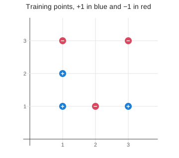
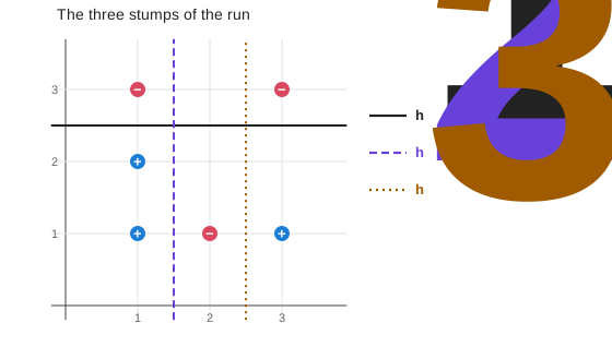
Six points: $(1,1)$, $(1,2)$, $(3,1)$ with label $+1$ and $(1,3)$, $(2,1)$, $(3,3)$ with label $-1$. The weak learners are decision stumps on one coordinate $j\in \{1,2\}$: $h(x)=s$ if $x^{(j)}>\theta$ and $-s$ otherwise, with $s\in \{\pm 1\}$ and $\theta \in \{1.5,2.5\}$. In every round the weak learner returns the stump with the smallest weighted error. The AdaBoost formulas are given: ${\epsilon }_t={\sum }_i{D}_i^{(t)}1[y_i\ne h_t(x_i)]$, $w_t=\frac{1}{2}\log (\frac{1}{{\epsilon }_t}-1)$, $D_i^{(t+1)}\propto D_i^{(t)}\exp (-w_t{y}_i{h}_t(x_i))$.

(a) (2 P, block A) Determine $h_1$, ${\epsilon }_1$ and $w_1$.

(b) (2 P, block A) Compute $D^{(2)}$, normalized, and check it.

(c) (3 P, block A) Determine $h_2$, ${\epsilon }_2$ and $w_2$.

(d) (3 P, blocks A and C) Give the combined classifier $\mathrm{sign}(w_1{h}_1+w_2{h}_2)$ on the six points and its training error. Compare with the bound $Z_2={\prod }_{t}2\sqrt{{\epsilon }_t(1-{\epsilon }_t)}$.

(e) (3 P, block A) Compute $D^{(3)}$. The third stump is $h_3$: $+1$ for $x^{(1)}>2.5$ and $-1$ otherwise. Compute ${\epsilon }_3$ and $w_3$ and the final classifier on all six points.

(f) (3 P, block B) Now take the XOR configuration $(1,1),(2,2)$ with label $+1$ and $(1,2),(2,1)$ with label $-1$. What happens in the first round, and why? And what does AdaBoost do with a stump that has ${\epsilon }_t>\frac{1}{2}$?

Solution

(a) With uniform weights $\frac{1}{6}$, count the mistakes of every stump. The stump ”$-1$ for $x^{(2)}>2.5$, $+1$ otherwise” only misclassifies $(2,1)$. Every other stump makes at least two mistakes. So $h_1$ is this stump, ${\epsilon }_1=\frac{1}{6}$ and $w_1=\frac{1}{2}\log 5\approx 0.805$. (2 P)

(b) The wrong point gets $D_i/(2{\epsilon }_1)=\frac{1}{6}\cdot 3=\frac{1}{2}$, every correct point $D_i/(2(1-{\epsilon }_1))=\frac{1}{6}\cdot \frac{3}{5}=\frac{1}{10}$. So $D^{(2)}$ is $\frac{1}{2}$ at $(2,1)$ and $\frac{1}{10}$ at the other five points. Check: $\frac{1}{2}+5\cdot \frac{1}{10}=1$, and the mistake carries exactly half of the weight. (2 P)

(c) Weighted errors under $D^{(2)}$, best orientation of each line:

Stump	Mistakes	Weighted error
$x^{(2)}>2.5\to -1$ (the old $h_1$)	$(2,1)$	$\frac{1}{2}$
$x^{(2)}>1.5\to +1$	$(1,1)$, $(3,1)$, $(1,3)$, $(3,3)$	$\frac{4}{10}$
$x^{(1)}>1.5\to -1$	$(3,1)$, $(1,3)$	$\frac{2}{10}$
$x^{(1)}>2.5\to +1$	$(1,1)$, $(1,2)$, $(3,3)$	$\frac{3}{10}$

So $h_2$: $+1$ for $x^{(1)}<1.5$ and $-1$ for $x^{(1)}>1.5$, with ${\epsilon }_2=\frac{1}{5}$ and $w_2=\frac{1}{2}\log 4\approx 0.693$. (3 P)

(d) $f_2=0.805h_1+0.693h_2$. Where the two stumps disagree, $h_1$ wins because its vote is larger.

Point	$y$	$h_1$	$h_2$	$f_2$	correct?
$(1,1)$	$+$	$+$	$+$	$1.498$	yes
$(1,2)$	$+$	$+$	$+$	$1.498$	yes
$(3,1)$	$+$	$+$	$-$	$0.112$	yes
$(1,3)$	$-$	$-$	$+$	$-0.112$	yes
$(2,1)$	$-$	$+$	$-$	$0.112$	no
$(3,3)$	$-$	$-$	$-$	$-1.498$	yes

Training error $\frac{1}{6}$. Bound: $Z_2=2\sqrt{\frac{1}{6}\cdot \frac{5}{6}}\cdot 2\sqrt{\frac{1}{5}\cdot \frac{4}{5}}=0.745\cdot 0.8\approx 0.60\ge \frac{1}{6}$. (3 P)

(e) Under $D^{(2)}$ the mistakes of $h_2$ are $(3,1)$ and $(1,3)$: each gets $\frac{1}{10}/(2\cdot \frac{1}{5})=\frac{1}{4}$. Correct points are divided by $2\cdot \frac{4}{5}=\frac{8}{5}$: $(2,1)$ gets $\frac{1}{2}\cdot \frac{5}{8}=\frac{5}{16}$, and $(1,1)$, $(1,2)$, $(3,3)$ get $\frac{1}{16}$ each. Check: $\frac{1}{4}+\frac{1}{4}=\frac{1}{2}$ and the total is 1. $h_3$ misclassifies $(1,1)$, $(1,2)$ and $(3,3)$: ${\epsilon }_3=\frac{3}{16}$ and $w_3=\frac{1}{2}\log \frac{13}{3}\approx 0.733$.

Final values $f_3=0.805h_1+0.693h_2+0.733h_3$: $(1,1)$ and $(1,2)$: $0.805+0.693-0.733=0.765$. $(3,1)$: $0.805-0.693+0.733=0.845$. $(1,3)$: $-0.805+0.693-0.733=-0.845$. $(2,1)$: $0.805-0.693-0.733=-0.622$. $(3,3)$: $-0.805-0.693+0.733=-0.765$. All six signs are right: training error 0 after three rounds, although every single stump makes mistakes. (3 P)

(f) Every stump cuts the square into two halves, and each half contains one $+$ and one $-$. So every stump has weighted error exactly $\frac{1}{2}$, the vote is $w_1=\frac{1}{2}\log 1=0$ and the weights stay uniform. Every later round finds the same situation: AdaBoost makes no progress, because the weak learning assumption ${\epsilon }_t\le \frac{1}{2}-\gamma$ fails. A stump with ${\epsilon }_t>\frac{1}{2}$ gets a negative vote, which is the same as using the flipped stump with error $1-{\epsilon }_t$. (3 P)

Full integration task: bagging, the bound and one gradient step (12 P)

Math: variance of an average · solving e^(-cT) < δ

(a) (2 P, block D) Each tree of an ensemble predicts at a fixed test point with variance ${\sigma }^2=9$ and bias 1. Any two trees have correlation $\rho =0.25$. Compute the variance of the average of $B=12$ trees and of $B\to \infty$ trees.

(b) (2 P, block D) How many trees bring the variance within 10% of its limit? Compare the expected squared error of the infinite ensemble with that of a single tree.

(c) (3 P, block C) AdaBoost runs on $n=500$ points, and every weak learner has weighted error at most $0.3$. Give $\gamma$, the bound on the training error after $T=20$ rounds, and the number of rounds after which the training error is guaranteed to be 0.

(d) (1 P, block C) How many rounds suffice with the sharper factor $2\sqrt{\epsilon (1-\epsilon )}$ per round?

(e) (2 P, block E) The test error of a boosted model keeps falling after the training error has reached 0. Which of the two test error bounds explains this, and which one gets worse with more rounds?

(f) (2 P, block E) Gradient boosting with the squared loss $\frac{1}{2}(y-\hat{y}{)}^2$ on three points with labels $y=(1,4,10)$, starting from the mean $f_0\equiv 5$. The next base function is a stump that separates the first two points from the third and predicts the mean of its targets on each side. Compute the targets, the stump and $f_1$ with step size 1.

Solution

(a) $\mathrm{Var}=\rho {\sigma }^2+(1-\rho )\frac{{\sigma }^2}{B}=0.25\cdot 9+0.75\cdot \frac{9}{12}=2.25+0.5625\approx 2.81$. For $B\to \infty$: $\rho {\sigma }^2=2.25$. (2 P)

(b) The part that still shrinks must be at most 10% of the limit: $\frac{0.75\cdot 9}{B}\le 0.225⟺B\ge 30$. Squared error of the infinite ensemble: $1^2+2.25=3.25$. A single tree: $1+9=10$. The bias stays, only the variance falls. (2 P)

(c) $\gamma =0.5-0.3=0.2$. After 20 rounds: $\exp (-2\cdot 0.04\cdot 20)=e^{-1.6}\approx 0.20$. The training error is a multiple of $\frac{1}{n}$, so it is 0 as soon as the bound is below $\frac{1}{500}$: $T>\frac{\ln 500}{2{\gamma }^2}=\frac{6.21}{0.08}\approx 77.7$, so $T=78$ rounds. (3 P)

(d) $2\sqrt{0.3\cdot 0.7}\approx 0.917$. $0.917^T<\frac{1}{500}⟺T>\frac{\ln 500}{-\ln 0.917}\approx \frac{6.21}{0.087}\approx 71.3$, so 72 rounds. (1 P)

(e) The margin bound explains it: it contains the VC dimension of the base class and the margin $\theta$, but not the number of rounds, and the margins can keep growing after the training error is 0. The VC bound uses $d=T\cdot d_{\mathcal{B}}$ and gets worse with every round. (2 P)

(f) For the squared loss the negative gradient is the residual $y_i-f_0(x_i)$: targets $(-4,-1,5)$. The stump predicts the mean on each side: $-2.5$ for the first two points and $5$ for the third. $f_1=f_0+h_1=(2.5,2.5,10)$, with the new residuals $(-1.5,1.5,0)$. (2 P)

Cheat sheet: bagging and boosting (6 blocks)

A. One round of AdaBoost by hand

1. Stump. For every candidate line and both orientations, add the weights of the points on the wrong side. Take the smallest sum: that is $h_t$ with error ${\epsilon }_t$.
2. Vote. $w_t=\frac{1}{2}\log \frac{1-{\epsilon }_t}{{\epsilon }_t}$.
3. New weights. A wrong point gets $\frac{D_i}{2{\epsilon }_t}$, a correct point $\frac{D_i}{2(1-{\epsilon }_t)}$. No exponentials needed.
4. Checks. The wrong points together have weight exactly $\frac{1}{2}$, and all weights add up to 1.
5. Combined classifier. One row per point with $h_1,h_2,\dots$ and the sum ${\sum }_t{w}_t{h}_t(x)$. Its sign is the prediction.

${\epsilon }_t$	vote $w_t$	factor $2\sqrt{{\epsilon }_t(1-{\epsilon }_t)}$
$\frac{1}{2}$	0	1
$0.4$	0.20	0.98
$\frac{1}{3}$	0.35	0.94
$\frac{1}{4}$	0.55	0.87
$\frac{1}{5}$	0.69	0.80
$\frac{1}{6}$	0.80	0.75
$0.1$	1.10	0.60

The factor is the amount by which one round multiplies the bound of block C.

B. Reading the plot and special cases

You see	It means
a stump as a line with a $+$ side and a $-$ side	its error is the weight of the points on the wrong side
the flipped stump	error $1-\epsilon$. Use whichever orientation is below $\frac{1}{2}$
a stump with ${\epsilon }_t=\frac{1}{2}$	vote 0, the weights do not change, no progress
every stump has one $+$ and one $-$ on each side (XOR)	$\epsilon =\frac{1}{2}$ for all stumps: boosting stumps fails, it needs deeper trees
a point with weight $\frac{1}{2}$	the next stump has to get it right, otherwise its error is at least $\frac{1}{2}$
the old stump under the new weights	error exactly $\frac{1}{2}$, so the next stump must be a different one
two stumps disagree at a point	the one with the larger vote decides

Left: the error of a stump is the weight of the circled points, the ones on the wrong side. Right: on XOR every stump is wrong on exactly half of the weight.

C. Training error bound

• Edge $\gamma =\frac{1}{2}-\epsilon$ (with the largest error of the weak learners).
• Training error $\le Z_T={\prod }_{t\le T}2\sqrt{{\epsilon }_t(1-{\epsilon }_t)}\le \exp (-2{\gamma }^{2}T)$.
• Zero training error is guaranteed once the bound is below $\frac{1}{n}$: $T>\frac{\ln n}{2{\gamma }^2}$, or with the sharper factor $T>\frac{\ln n}{-\ln \left(2\sqrt{\epsilon (1-\epsilon )}\right)}$. Round up.

D. Bagging

$$\mathrm{Var}(\text{average of }B)=\rho {\sigma }^2+(1-\rho )\frac{{\sigma }^2}{B}$$

• Independent ($\rho =0$): ${\sigma }^2/B$. Limit for $B\to \infty$: $\rho {\sigma }^2$.
• Within a fraction $q$ of the limit: $B\ge \frac{1-\rho }{q\rho }$.
• The bias does not change. Squared error $=$ bias${}^2$ $+$ variance.
• A bootstrap sample misses a fixed point with probability $(1-\frac{1}{n}{)}^n\approx 0.37$.

E. Test error and the three methods

You see	It means
VC bound with $d=T\cdot d_{\mathcal{B}}$	gets worse with every round, needs $T/n\to 0$
margin bound	$T$ does not appear: the test error can fall after the training error is 0
deep trees, averaged in parallel	bagging or random forest: lowers the variance
stumps, added one after the other with votes	boosting: lowers the bias
gradient boosting with the squared loss	the next tree is fitted to the residuals $y_i-f_{t-1}(x_i)$

F. Traps

• Normalize the new weights. With the shortcut of block A they already add up to 1.
• Use the weighted error under the current $D^{(t)}$, not the number of mistakes.
• The combined classifier is the sign of the weighted sum, not a majority of the stumps.
• The bound $Z_T$ can be far above the true training error. It is still a valid check.
• Bagging cannot repair a bias, and its variance does not go to 0 if the trees are correlated.

References

All sources cited on the slides, in slide order (19 entries)

Slide	Source	Key point
4	Hastie, Tibshirani and Friedman, The Elements of Statistical Learning (online)	statistics view of ensembles
9	Efron and Tibshirani, An Introduction to the Bootstrap	standard bootstrap textbook
9	Shao and Tu, The Jackknife and Bootstrap	mathematical treatment
13	Breiman, “Random forests”, Machine Learning, 2001	original random forest paper
13	Biau and Scornet, “A random forest guided tour”, Test 25(2):197-227, 2016	overview
13	Hastie, Tibshirani and Friedman, Ch. 8, 9, 15; Shalev-Shwartz and Ben-David, Ch. 18	textbooks
13, 22, 24	Tang, Garreau and von Luxburg, “When do random forests fail?”, NeurIPS 2018	failure regimes of forests
13, 26	Haghiri, Garreau and von Luxburg, “Comparison-Based Random Forests”, ICML 2018	comparison trees
21	Hastie, Tibshirani and Friedman, Algorithm 15.1	random forest pseudocode
23	Biau, “Analysis of a random forests model”, JMLR, 2012	consistent trees give a consistent forest
24	Scornet, “On the asymptotics of random forests”, Journal of Multivariate Analysis, 2016	forests of inconsistent deep trees
27	Shalev-Shwartz and Ben-David, Understanding Machine Learning, Sec. 10 (online)	boosting
27, 32-35, 56	Schapire and Freund, Boosting: Foundations and Algorithms	boosting book, toy example, margin bound
27	Schapire and Freund, 1995	original AdaBoost paper
38	Understanding Machine Learning	AdaBoost pseudocode
44	Shalev-Shwartz and Ben-David Sec. 10; Schapire and Freund Sec. 3.1	proof details of Theorem 1 (training error of AdaBoost)
59	Schapire and Freund, Sec. 4.3	weak = strong learnability
60	Friedman, “Greedy Function Approximation: A Gradient Boosting Machine”, Annals of Statistics, 2001	gradient boosting
60	Chen and Guestrin, “XGBoost: A Scalable Tree Boosting System”, KDD 2016	XGBoost

Related

• Previous: Lecture 5: Regularization · Next: Lecture 7: Data, Measurement and Validity · Course: Overview · Formula Sheet · Glossary
• Concepts: Bagging, Random Forest, AdaBoost, Gradient Boosting, Surrogate Loss (exponential loss), VC Dimension, Margin
• Exercises: Sheet 7, Exercise 3 (why bagging reduces variance); Sheet 8 (AdaBoost with stumps by hand and implemented, gradient boosting)