Lecture 5: Regularization

TL;DR

1. Regularization minimizes the regularized risk $R_{reg,n}(f)=R_n(f)+\lambda \Omega (f)$ with a regularizer $\Omega$ that measures how “complex” $f$ is. It controls the size of the function class implicitly: a large $\lambda$ means a solution in a small class ${\mathcal{F}}_t=\{\Omega (f)\le t\}$. For consistency, let ${\lambda }_n\to 0$ slowly.
2. Least squares ${\min }_w\Vert Y-Xw{\Vert }^2$: if $\mathrm{rank}(X)=d$, $w=(X^{t}X{)}^{-1}{X}^{t}Y$ is unique. Otherwise $w=(X^{t}X{)}^{+}{X}^{t}Y$ with the generalized inverse, and every $w+v$ with $Xv=0$ is also a solution: all agree on the training points but not on test points.
3. Ridge regression ${\min }_w\frac{1}{n}\Vert Y-Xw{\Vert }^2+\lambda \Vert w{\Vert }^2$ has the unique solution $w_{n,\lambda }=(X^{t}X+n\lambda I_d{)}^{-1}{X}^{t}Y$ for every $\lambda >0$. Via the SVD it shrinks the directions with small singular values (mostly noise) the most.
4. $\lambda \Vert w{\Vert }^2$ is $2\lambda$-strongly convex, so ridge (with a convex $L$-Lipschitz loss) is uniformly stable with ${\Delta }_{\sup }\le 2L^2/(\lambda n)$: regularization implies stability (Lecture 4).
5. Lasso ${\min }_w\frac{1}{n}\Vert Y-Xw{\Vert }_2^2+\lambda \Vert w{\Vert }_1$: $\Vert w{\Vert }_1$ is the convex norm closest to the (NP-hard) count $\Vert w{\Vert }_0$, and its corners give sparse solutions. No closed form.
6. Rates (fixed design, excess risk): OLS ${\sigma }^{2}d/n$ (fast rate, bad in $d$); ridge $\sigma \Vert {\theta }^{\ast }{\Vert }_2\sqrt{d}/\sqrt{n}$; lasso $\sigma k\sqrt{\log d}/\sqrt{n}$; $L_0$ ${\sigma }^{2}k\log d/n$ for $k$-sparse ${\theta }^{\ast }$. Sparsity turns the dependence on $d$ into $\log d$.

Exam relevance

Neither the first exam nor the mock asked about this lecture directly, so it is a candidate for new tasks in the retake. Likely formats:

• Multiple choice: effect of $\lambda$ on bias, variance, approximation and estimation error; why the lasso is sparse and ridge is not; which norms are convex; which rate belongs to which regularizer.
• Computations: ridge and lasso by hand for an orthogonal design (task), the closed form of ridge for small data.
• Selecting rates (task type 4 of the real exam): which regularizer has the best bound for given $n$, $d$, $k$ (task).
• Stability rates (task type 7): how fast ${\lambda }_n$ may go to 0 so that the stability bound still vanishes (task).
• Sheet 6: normal equations via orthogonality, over- and underdetermined regime, minimum norm interpolant, ridge as OLS on an augmented system, why ${\ell }_1$ gives sparse solutions.
• Everything in one go: the cheat sheet with two full integration tasks at the end of this note.

Exam essentials (6 cards)

Only what you should know by heart in the exam. Click a card for the answer, or press a to go through them as flashcards. For Anki: deck of this lecture.

Regularized risk, and what does $\lambda$ do?

Answer

$R_{reg,n}(f)=R_n(f)+\lambda \Omega (f)$.
Large $\lambda$: small class $\{\Omega (f)\le t\}$, stable but biased. For consistency let ${\lambda }_n\to 0$ slowly.

Least squares solution, with and without full rank?

Answer

$\mathrm{rank}(X)=d$: $w=(X^{t}X{)}^{-1}{X}^{t}Y$, unique.
Otherwise $w=(X^{t}X{)}^{+}{X}^{t}Y$, and every $w+v$ with $Xv=0$ is also a solution.

Ridge regression: problem and solution?

Answer

${\min }_w\frac{1}{n}\Vert Y-Xw{\Vert }^2+\lambda \Vert w{\Vert }^2$
$w_{n,\lambda }=(X^{t}X+n\lambda I_d{)}^{-1}{X}^{t}Y$, unique for every $\lambda >0$.

Lasso: problem, and how does it differ from ridge?

Answer

${\min }_w\frac{1}{n}\Vert Y-Xw{\Vert }_2^2+\lambda \Vert w{\Vert }_1$, no closed form.
Lasso sets coefficients exactly to 0 (sparse), ridge only shrinks them.

Why does regularization imply stability?

Answer

$\lambda \Vert w{\Vert }^2$ is $2\lambda$-strongly convex, so with a convex $L$-Lipschitz loss ${\Delta }_{\sup }\le \frac{2L^2}{\lambda n}$.

Excess risk rates of OLS, ridge, lasso and $L_0$?

Answer

OLS ${\sigma }^{2}d/n$; ridge $\sigma \Vert {\theta }^{\ast }{\Vert }_2\sqrt{d}/\sqrt{n}$; lasso $\sigma k\sqrt{\log d}/\sqrt{n}$; $L_0$: ${\sigma }^{2}k\log d/n$.
Sparsity turns the dependence on $d$ into $\log d$.

Overview: 1. The principle of regularization, 2. Recap: linear least squares, 3. Ridge regression, 4. Tikhonov regularization leads to stability, 5. Lasso and sparsity, 6. Theoretical results for the different regularizers.

Explicit regularization

The principle of regularization

Slides 3-7

(Literature: Shalev-Shwartz and Ben-David, Understanding Machine Learning, Sec. 13.)

• Training set of $n$ points in the standard setup, $\mathcal{F}$ a very large space of functions (say all real-valued differentiable functions), a loss $\ell$ with empirical and true risk $R_n$ and $R$.

Regularizer and regularized risk

A regularizer $\Omega :\mathcal{F}\to {\mathbb{R}}_{\ge 0}$ measures how “complex” a function is. Examples: $\mathcal{F}$ = polynomials, $\Omega (f)$ = degree of $f$; $\mathcal{F}$ = differentiable functions, $\Omega (f)$ = maximal slope. The regularized risk is

$$R_{reg,n}(f):=R_n(f)+\lambda \cdot \Omega (f)$$

with the regularization constant $\lambda >0$. Choose $f\in \mathcal{F}$ to minimize the regularized risk on the training data.

Why it makes sense

• If a “simple” function fits the data reasonably well, choose it. If all simple functions have a very high empirical risk, choose a more complex one.
• SLT (Lecture 3) says: control the size of the function class. In practice this is difficult to do explicitly; regularization does it implicitly, because spaces of simple functions have smaller capacity.
• Nice side effects: the solution may become unique, the optimization problem may become easier, and the algorithm may become stable, with better generalization guarantees.

What can we choose as a regularizer?

Slides 8-10

Regularizers enforce properties that are hard to control otherwise, such as sparsity or interpretability. $\Omega$ takes the parameters of the function as input and returns a real number that measures the property (the smaller the better, since we minimize); to use gradient methods it should be differentiable.

The trade-off: nested function spaces

Consider ${\mathcal{F}}_t:=\{f\in \mathcal{F}\mid \Omega (f)\le t\}$, nested in $t$.

• $\lambda$ small ⇝ the solution lies in ${\mathcal{F}}_t$ with $t$ large: a rich class, small approximation error, large estimation error, risk of overfitting.
• $\lambda$ large ⇝ the solution lies in ${\mathcal{F}}_t$ with $t$ small: a poor class, large approximation error, small estimation error, risk of underfitting.
• $\lambda =0$ is plain ERM over $\mathcal{F}$.

But we changed the objective!

Slides 11-12

Regularization does change the objective we optimize. So what about consistency? The idea:

• choose a huge function class $\mathcal{F}$ that definitely contains the Bayes classifier;
• while $n$ is small, use a large regularization constant ${\lambda }_n$ (do not overfit with a complex function);
• as $n$ grows, slowly decrease ${\lambda }_n$: we need (and can afford) more complex functions, and still prevent overfitting;
• as $n\to \infty$, ${\lambda }_n\to 0$ (at a rate to be determined): in the infinite-sample limit we essentially do not regularize and pick the best function in $\mathcal{F}$, the Bayes classifier.

To prove consistency one has to show that this framework works, i.e. $f_n$ converges to $f^{\ast }$. (The stability argument below gives one way.)

Recap: linear least squares regression

Linear setup and concise notation

Slides 13-19

(Literature: Shalev-Shwartz and Ben-David Sec. 9, Bach Sec. 3.)

Training data $(X_i,Y_i)$ with $X_i\in {\mathbb{R}}^d$ and $Y_i\in \mathbb{R}$. We look for the best linear function $f(x)={\sum }_{i=1}^d{w}_i{x}^{(i)}+b$ (weights $w_i$, offset or intercept $b$) under the squared loss:

$$\underset{w,b}{\min }\frac{1}{n}\sum _{i=1}^n(Y_i-f(X_i){)}^2$$

Matrix notation

Stack the inputs as rows of the design matrix $X\in {\mathbb{R}}^{n\times d}$ ($X_{ik}$ = $k$-th coordinate of point $i$), the outputs in $Y\in {\mathbb{R}}^n$, the weights in $w\in {\mathbb{R}}^d$. Then $f(X_i)=⟨X_i,w⟩+b=(Xw{)}_i+b$.

Getting rid of $b$: append a column of ones to $X$ and $b$ to $w$: $\tilde{X}=[X1]\in {\mathbb{R}}^{n\times (d+1)}$, $\tilde{w}=(w_1,\dots ,w_d,b)$. Then $(\tilde{X}\tilde{w}{)}_i=(Xw{)}_i+b$, and the problem becomes ${\min }_{\tilde{w}}\frac{1}{n}\Vert Y-\tilde{X}\tilde{w}{\Vert }^2$.

From now on (without loss of generality, dropping the tildes): ${\min }_{w\in {\mathbb{R}}^d}\Vert Y-Xw{\Vert }^2$.

Proposition 1 (least squares is convex)

The least squares problem is a convex optimization problem. (Proof: exercise. The Hessian $X^{t}X$ is positive semi-definite.)

Solution in the full rank case

Slides 20-21

Theorem 2 (solution, case $\mathrm{rank}(X)=d$)

If $X$ has rank $d$, the solution of linear least squares is

$$w=(X^{t}X{)}^{-1}{X}^{t}Y$$

Proof

Objective $Obj(w):=\frac{1}{2}\Vert Y-Xw{\Vert }^2$, gradient $\nabla Obj(w)=-X^t(Y-Xw)$. Setting it to zero gives the normal equations $X^{t}Y=(X^{t}X)w$. We always have $\mathrm{rank}(X)=\mathrm{rank}(X^{t}X)=\mathrm{rank}(X{X}^t)$, so for $\mathrm{rank}(X)=d$ the $d\times d$ matrix $X^{t}X$ is invertible and $w=(X^{t}X{)}^{-1}{X}^{t}Y$.

Minimum: the Hessian is $X^{t}X$. It is positive semi-definite ($v^t{X}^{t}Xv=\Vert Xv{\Vert }^2\ge 0$), and because of the rank condition all eigenvalues are $>0$. $\square$

Mini example

Three points $(x,y)$: $(1,1)$, $(2,2)$, $(3,2)$, no intercept, $d=1$. $X^{t}X=1+4+9=14$, $X^{t}Y=1+4+6=11$, so $w=11/14\approx 0.786$.

Generalized inverse and the general case

Slides 22-25

Moore-Penrose generalized inverse

A symmetric $A\in {\mathbb{R}}^{d\times d}$ with eigenvalues ${\lambda }_i$ and eigenvectors $v_i$ has the spectral decomposition $A={\sum }_{i=1}^d{\lambda }_i{v}_i{v}_i^t$. If all ${\lambda }_i\ne 0$, $A^{-1}={\sum }_i\frac{1}{{\lambda }_i}{v}_i{v}_i^t$. If $A$ is not of full rank, the generalized inverse is

$$A^{+}:=\sum _{i:{\lambda }_i\ne 0}\frac{1}{{\lambda }_i}{v}_i{v}_i^t$$

Intuitively, the inverse of $A$ restricted to the subspace orthogonal to its nullspace. In general $A{A}^{+}\ne I$, but $A{A}^{+}A=A$ and $A^{+}A{A}^{+}=A^{+}$; if $A$ is invertible, $A^{+}=A^{-1}$.

Theorem 3 (solution, case $\mathrm{rank}(X)<d$)

1. A solution of linear least squares is $w=(X^{t}X{)}^{+}{X}^{t}Y$.
2. It is not unique. But any two solutions $w_1,w_2$ agree on the training data: $⟨w_1,X_i⟩=⟨w_2,X_i⟩$ for all $i$.

Proof sketch

As before the normal equations $X^{t}Y=(X^{t}X)w$ are necessary; one checks that $w=(X^{t}X{)}^{+}{X}^{t}Y$ satisfies them (exercise). Non-uniqueness: since $\mathrm{rank}(X)<d$ there is $v\ne 0$ with $Xv=0$, and $w+v$ is a solution with the same objective value. Predictions on the training points: $X(w_1+v)=X{w}_1+Xv=X{w}_1$. $\square$

On test points the solutions disagree. Which one to prefer? One idea is regularization (below); another is the minimum norm solution (Sheet 6, Lecture 8).

Relationship between n and d

Slides 26-29

The linear system $X^{t}Y=(X^{t}X)w$ has $d$ equations and $d$ unknowns, independently of $n$. Either the solution is unique ($\mathrm{rank}(X^{t}X)=d$) or there are many ($\mathrm{rank}<d$); a solution always exists, however large $n$ is. Informally, $d$ is the number of parameters, $n$ the number of constraints.

• $d\ll n$: harmless. Many points in a low-dimensional space; linear functions are not very flexible and we tend not to overfit (sometimes we underfit). This is what classical statistics has treated for a century.
• $d\gg n$: not quite as harmless. Few points in a high-dimensional space make linear functions very powerful: the function class is too large, which often leads to overfitting. But sometimes “benign overfitting” takes place, particularly in linear regression: the inductive bias of the algorithm makes it harmless (Lecture 8). Many surprising things happen for $d\gg n$ (high-dimensional statistics: Wainwright; Bühlmann and van de Geer).

Ridge regression (Tikhonov regularization)

Idea and problem

Slides 30-32

(Literature: Bach Sec. 3.6, Shalev-Shwartz and Ben-David Sec. 13.1, Hastie, Tibshirani and Friedman Sec. 3.4.3.) Two goals:

1. a unique solution, whatever the rank of the design matrix (numerical stability);
2. small coefficients: in plain least squares the $w_i$ can become very large, which gives a high variance of the results.

Ridge regression

With the regularizer $\Omega (f)=\Vert w{\Vert }^2={\sum }_{i=1}^d{w}_i^2$ and $\lambda >0$:

$$w_{n,\lambda }:=\underset{w\in {\mathbb{R}}^d}{\mathrm{argmin}}\frac{1}{n}\Vert Y-Xw{\Vert }^2+\lambda \Vert w{\Vert }^2$$

Solution of ridge regression

Slides 33-35

Theorem 4 (solution of ridge regression)

$$w_{n,\lambda }=(X^{t}X+n\lambda I_d{)}^{-1}{X}^{t}Y$$

The matrix is invertible for every $\lambda >0$, so the solution always exists and is unique.

Proof

$Obj(w)=\frac{1}{n}\Vert Y-Xw{\Vert }^2+\lambda \Vert w{\Vert }^2$ is convex. Setting the gradient to zero:

$$\nabla Obj(w)=-\frac{2}{n}{X}^t(Y-Xw)+2\lambda w\stackrel{!}{=}0⟹(X^{t}X+n\lambda I_d)w_{n,\lambda }=X^{t}Y$$

Invertibility. $A:=X^{t}X$ is symmetric positive semi-definite, so all its eigenvalues $\sigma \ge 0$. If $Av=\sigma v$, then $(A+cI)v=(\sigma +c)v$: the eigenvalues of $A+cI$ are $\sigma +c>0$ for $c=n\lambda >0$. So $A+n\lambda I$ has full rank. $\square$

Mini example (the data from above)

Points $(1,1)$, $(2,2)$, $(3,2)$, $n=3$, $\lambda =1$: $w=\frac{X^{t}Y}{X^{t}X+n\lambda }=\frac{11}{14+3}\approx 0.647$ instead of $0.786$. The coefficient is shrunk towards 0.

Memory aid

Ridge adds $n\lambda$ to every eigenvalue: the matrix is always invertible, and directions with small eigenvalues (mostly noise) are shrunk the most.

Choice of the parameter λ

Slides 36-38

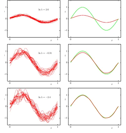
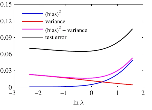
Question: what is the role of $\lambda$, and what happens to the estimation and approximation error if it is high or low? Larger $\lambda$ gives less complex functions: bias goes up, variance goes down.

Slide 37 (from Bishop's book): left, fits on many data sets for decreasing regularization (ln λ = 2.6, −0.31, −2.4); right, the true curve (green) and the average fit (red).

Slide 38: bias², variance and test error against ln λ.

(*) Ridge regression as a shrinkage method

Slides 39-42

With the singular value decomposition $X=U\Sigma V^t$ (singular values ${\sigma }_j$), plugging into the formula gives (absorbing the factor $n$ into $\lambda$)

$$w_{n,\lambda }=V\mathrm{diag}\left(\frac{{\sigma }_j}{{\sigma }_j^2+\lambda }\right)U^{t}Y$$

• Without regularization ($\lambda =0$): $\frac{{\sigma }_j}{{\sigma }_j^2+0}=\frac{1}{{\sigma }_j}$.
• Large ${\sigma }_j$: $\frac{{\sigma }_j}{{\sigma }_j^2+\lambda }\approx \frac{1}{{\sigma }_j}$, not much difference.
• Small ${\sigma }_j$: $\frac{{\sigma }_j}{{\sigma }_j^2+\lambda }\ll \frac{1}{{\sigma }_j}$.

Intuition

Regularization “shrinks” the directions of small variance. These are the directions that mainly contain noise, not signal. In statistics such methods are called shrinkage methods.

Stein's paradox and the James-Stein estimator

Estimate the mean $\theta$ of $N(\theta ,I)$ in ${\mathbb{R}}^d$, $d\ge 3$, from a single data point $X$. The least squares estimator is ${\hat{\theta }}_{LS}=X$. The shrinkage estimator

$${\hat{\theta }}_{JS}=(1-\frac{d-2}{\Vert X{\Vert }^2})X$$

is better in expected error: $E(\Vert \theta -{\hat{\theta }}_{LS}\Vert )\ge E(\Vert \theta -{\hat{\theta }}_{JS}\Vert )$. Stein’s paradox (1950s): when estimating at least three parameters jointly, it is better to shrink them.

History and terminology

Slides 43-44

• Invented by Andrey Tikhonov, 1943, in the context of integral equations (“On the stability of inverse problems”, Doklady Akademii Nauk SSSR): hence Tikhonov regularization.
• Introduced in statistics by Hoerl and Kennard, “Ridge regression: Biased estimation for nonorthogonal problems”, Technometrics 1970.
• The original intention was to make the least squares solution more stable and unique: replace $X^{t}X$ by $X^{t}X+\lambda I$, adding a little “ridge” on the diagonal of the matrix. The regularization interpretation is more recent.

Tikhonov regularization leads to stability

Strong convexity from the regularizer

Slides 45-46

(Literature: Shalev-Shwartz and Ben-David Sec. 13.3; Hardt and Recht p. 113.) A convex loss (for example least squares on a bounded parameter domain) is nice, but convexity does not guarantee a rate for the optimizer, nor stability. For that we need strong convexity (Lecture 4), and the Tikhonov regularizer provides it.

Proposition 5 (the regularizer is strongly convex)

• $f(w)=\lambda \Vert w{\Vert }^2$ is $2\lambda$-strongly convex.
• If $g$ is convex and $f$ is $\mu$-strongly convex, then $f+g$ is $\mu$-strongly convex.

(Proof: exercise. The Hessian of $\lambda \Vert w{\Vert }^2$ is $2\lambda I$.)

Regularized ERM is stable

Slides 47-48

Stability of Tikhonov-regularized ERM

ERM with a $\mu$-strongly convex, $L$-Lipschitz loss has ${\Delta }_{\sup }\le \frac{4L^2}{\mu n}$ (Theorem 3: ERM is stable from Lecture 4). A convex loss plus $\lambda \Vert w{\Vert }^2$ is $\mu$-strongly convex with $\mu =2\lambda$, so

$${\Delta }_{\sup }\le \frac{2L^2}{\lambda n},E(R(f_n)-R_n(f_n))\le {\Delta }_{\sup }\le \frac{2L^2}{\lambda n}$$

Trap

Slide 47 writes the gap as $E(R_n(f_n)-R(f_n))$. The expected generalization gap in Proposition 1 (gap = average stability) of Lecture 4 is true minus empirical risk, $E(R(f_n)-R_n(f_n))$.

Choice of $\lambda$ (the trade-off again). The theorem holds for every fixed $\lambda$, but:

• the stability term ${\Delta }_{\sup }$, and with it the generalization gap, gets smaller as $\lambda$ increases;
• the empirical risk $R_n(f_n)$ gets larger as $\lambda$ increases, because the objective is less focused on a small empirical risk.

Which value to choose is not obvious. In practice one often uses cross validation; theory gives rules of thumb (see the bounds below).

Task: how fast may lambda go to zero?

Exam-style task: regularization, stability and rates (4 P)

Math: deciding whether a rate goes to 0

Regularized ERM with a convex, $L$-Lipschitz loss bounded by $M$ and the regularizer ${\lambda }_n\Vert w{\Vert }^2$. Use ${\Delta }_{\sup }\le 2L^2/({\lambda }_{n}n)$ and the stability bound $R\le R_n+{\beta }_n+(2n{\beta }_n+M)\sqrt{\log (1/\delta )/(2n)}$ of Lecture 4.

${\lambda }_n$	$1$	$n^{-1/4}$	$n^{-1/2}$	$n^{-1}$
gap → 0?
${\lambda }_n\to 0$?

(a) (1 P, easy) Compute ${\beta }_n$ for each ${\lambda }_n$.

(b) (1.5 P, harder) Fill in both rows of the table.

(c) (1.5 P, transfer) Which choices are candidates for a consistent regularization scheme, and why do you need both rows?

Solution

(a) ${\beta }_n=2L^2/({\lambda }_{n}n)$: $2L^2/n$, $2L^2{n}^{-3/4}$, $2L^2{n}^{-1/2}$, $2L^2$. (1 P)

(b) The gap vanishes iff $\sqrt{n}{\beta }_n\to 0$ iff ${\lambda }_n\sqrt{n}\to \infty$: yes for $1$ and $n^{-1/4}$, no for $n^{-1/2}$ (constant) and $n^{-1}$ (${\beta }_n$ does not even go to 0). ${\lambda }_n\to 0$: no for $1$, yes for the others. (1.5 P)

(c) Only ${\lambda }_n=n^{-1/4}$ satisfies both: the gap between training and test risk vanishes (stability) and the regularization disappears asymptotically, so the approximation error can go to 0 (slides 11-12). ${\lambda }_n=1$ generalizes but stays biased; ${\lambda }_n=n^{-1}$ removes the bias too quickly to be stable. In general ${\lambda }_n\to 0$ with ${\lambda }_n\sqrt{n}\to \infty$. (1.5 P)

Lasso: least squares with L1-regularization

Sparsity and a naive regularizer

Slides 49-52

(Books: Hastie, Tibshirani and Friedman Sec. 3.4.3; Bishop Sec. 3; Hastie, Tibshirani and Wainwright Sec. 2. Original paper: Tibshirani, “Regression shrinkage and selection via the lasso”, J. Royal Statist. Soc. B, 1996.)

In linear regression it is very desirable to obtain a solution where many coefficients $w_i$ are zero: a sparse solution. Reasons: stability of the solution; computational reasons (with many basis functions we only need to evaluate a few); interpretability.

Naive regularizer for sparsity

$${\Omega }_0(f):=\sum _{i=1}^d{1}_{w_i\ne 0}$$

directly penalizes the number of non-zero entries. But ${\Omega }_0$ is a discrete function, and optimizing discrete functions is typically NP hard.

Excursion: p-norms

Slides 53-55

p-norms and the zero-"norm"

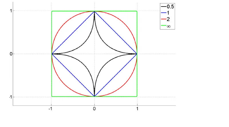
For $p>0$ and $w\in {\mathbb{R}}^d$: $\Vert w{\Vert }_p:=({\sum }_{i=1}^d|w_i{|}^p{)}^{1/p}$.

• For $p\ge 1$ this is a norm, hence a convex function.
• For $0<p<1$ it is not a norm and not convex.
• For $p=0$: $\Vert w{\Vert }_0:={\lim }_{p\to 0}\Vert w{\Vert }_p^p={\sum }_i|w_i{|}^0={\sum }_i{1}_{w_i\ne 0}={\Omega }_0(f)$ (with $0^0:=0$; the limit is of $\Vert w{\Vert }_p^p$, not of $\Vert w{\Vert }_p$). Not a norm (not even homogeneous), but called the zero-norm in the literature.

Slide 54: unit spheres for p = 0.5, 1, 2 and ∞. For p < 1 the ball is not convex.

Sparsity and the L1-norm

Slides 56-58

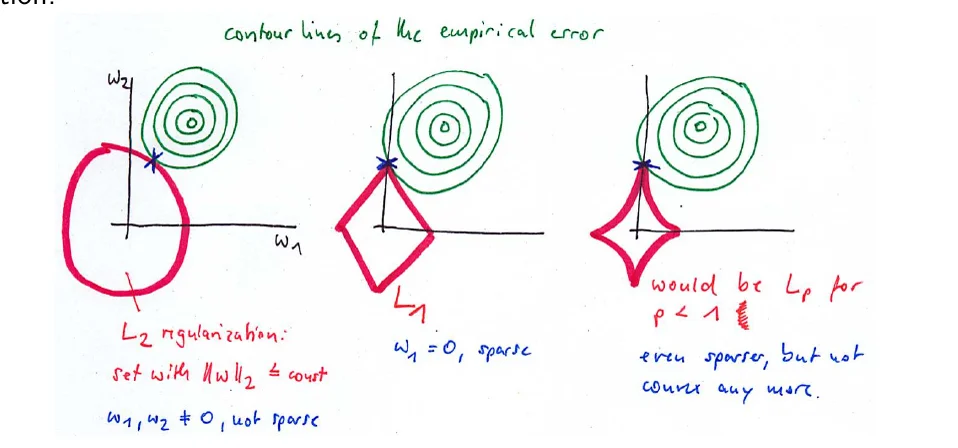
$\Vert w{\Vert }_1$ is “as close” to the non-convex $\Vert w{\Vert }_0$ as possible while still being convex. Does it still tend to give sparse solutions? Yes.

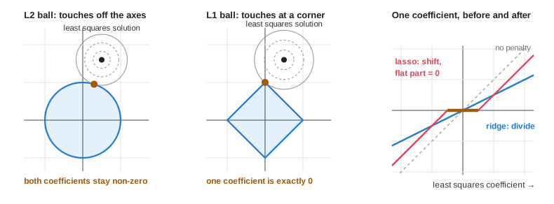
Slide 57: the best solution with ‖w‖ ≤ const. L2: both coordinates non-zero. L1: the contour lines touch at a corner, w₁ = 0 (sparse). Lp with p < 1: even sparser, but not convex any more.

Why L2 is not sparse and L1 is

The $L_2$-norm puts a particularly large (quadratic) penalty on large coefficients. To avoid it, it is better to have many small non-zero $w_i$ than a couple of large ones and many zeros: $L_2$ rather prevents sparsity. The $L_1$-norm punishes all weights linearly, so it can afford one large weight if at the same time many small weights disappear.

The picture of slide 57 to play with. Click to move the least squares solution ŵ, shrink the budget t and watch where the error ellipses touch the L2 ball (red) and the L1 diamond (blue). Right: the coefficient paths; lasso coefficients hit exactly 0, ridge coefficients only shrink.

The lasso

Slides 59-62

Lasso

Input space $\mathcal{X}\subset {\mathbb{R}}^d$, output $\mathcal{Y}=\mathbb{R}$, training data $X\in {\mathbb{R}}^{n\times d}$, $Y\in {\mathbb{R}}^n$, linear functions, squared loss, regularizer $\Omega (f)=\Vert w{\Vert }_1={\sum }_i|w_i|$:

$$w_{n,\lambda }:=\underset{w\in {\mathbb{R}}^d}{\mathrm{argmin}}\frac{1}{n}\Vert Y-Xw{\Vert }_2^2+\lambda \Vert w{\Vert }_1$$

The objective is convex (a sum of two convex functions), but there is no closed form solution; it is solved by a standard convex optimization algorithm.

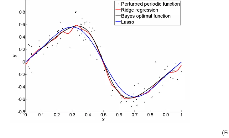
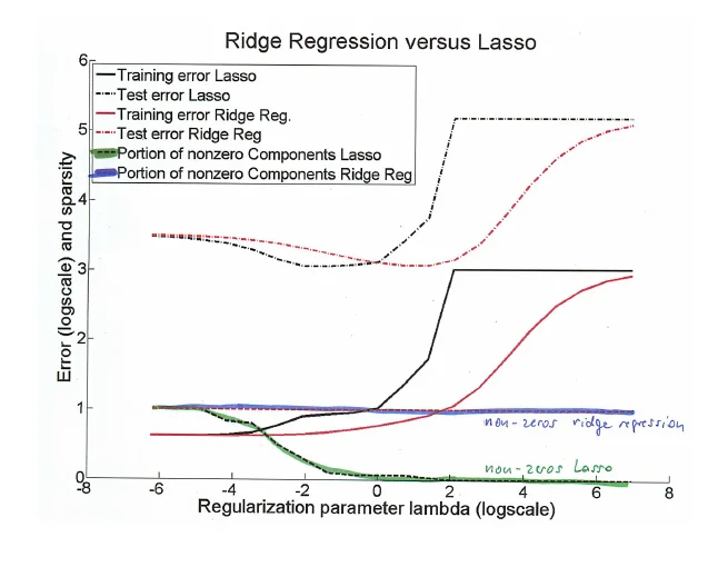
Slide 61 (figure by Matthias Hein): ridge and lasso fits of a perturbed periodic function.

Slide 60 (figure by Matthias Hein): with growing λ the lasso quickly sets almost all coefficients to 0 (green), ridge keeps all of them non-zero (blue). As the sparsity increases, the test error also increases rapidly.

History. LASSO stands for “least absolute shrinkage and selection operator”, invented by Tibshirani (1996); a short retrospective with literature pointers: Tibshirani, “Regression shrinkage and selection via the lasso: a retrospective”, J. R. Statist. Soc. B (2011).

Memory aid

Lasso = soft threshold: coefficients below $\lambda /2$ (orthogonal design) die, the others shrink by $\lambda /2$. Ridge only divides, it never kills.

Task: ridge and lasso by hand

Exam-style task: ridge and lasso for an orthogonal design (4 P)

Math: derivatives, also of the absolute value · ℓ1 and ℓ2 norms

Assume the columns of $X\in {\mathbb{R}}^{n\times 3}$ are orthogonal with $X^{t}X=n{I}_3$, and the unregularized least squares solution is $\hat{w}=\frac{1}{n}{X}^{t}Y=(2.0,0.3,-0.8)$. Then (up to a constant) $\frac{1}{n}\Vert Y-Xw{\Vert }^2=\Vert w-\hat{w}{\Vert }^2+\text{const}$.

(a) (1 P, easy) Show that ridge with $\lambda \Vert w{\Vert }^2$ gives $w_j={\hat{w}}_j/(1+\lambda )$, and compute it for $\lambda =1$.

(b) (1.5 P, harder) Show that the lasso with $\lambda \Vert w{\Vert }_1$ gives the soft thresholding $w_j=\mathrm{sign}({\hat{w}}_j)\max (|{\hat{w}}_j|-\lambda /2,0)$, and compute it for $\lambda =1$.

(c) (1.5 P, transfer) For which $\lambda$ is exactly one lasso coefficient non-zero? Can ridge ever produce a zero coefficient here?

Solution

(a) The objective separates per coordinate: $(w_j-{\hat{w}}_j{)}^2+\lambda w_j^2$, derivative $2(w_j-{\hat{w}}_j)+2\lambda w_j=0$, so $w_j={\hat{w}}_j/(1+\lambda )$. For $\lambda =1$: $(1.0,0.15,-0.4)$. (1 P)

(b) Per coordinate: $(w_j-{\hat{w}}_j{)}^2+\lambda |w_j|$. For $w_j>0$ the derivative $2(w_j-{\hat{w}}_j)+\lambda =0$ gives $w_j={\hat{w}}_j-\lambda /2$, valid if ${\hat{w}}_j>\lambda /2$; symmetric for $w_j<0$; otherwise the minimum is at the kink $w_j=0$. For $\lambda =1$ (threshold $0.5$): $(1.5,0,-0.3)$. (1.5 P)

(c) Coefficient $j$ is non-zero iff $|{\hat{w}}_j|>\lambda /2$. Exactly one (the first) survives iff $0.8\le \lambda /2<2$, i.e. $1.6\le \lambda <4$. Ridge only divides by $1+\lambda$, so a coefficient is 0 only if ${\hat{w}}_j=0$: ridge shrinks but does not select. (1.5 P)

Theoretical results for the different regularizers

Model assumptions: linear model plus noise

Slides 63-65

(Literature: Bach Sec. 3 for least squares without regularization and ridge, Sec. 8 for the lasso. The bounds are stated without proofs.) To make the analysis simpler, we make strong assumptions.

Linear model

Data $X_1,\dots ,X_n\in {\mathbb{R}}^d$ and a vector ${\theta }^{\ast }\in {\mathbb{R}}^d$ with

$$Y_i=⟨X_i,{\theta }^{\ast }⟩+{\epsilon }_i$$

where the noise variables ${\epsilon }_i\in \mathbb{R}$ are independent with $E({\epsilon }_i)=0$ and variance $E({\epsilon }_i^2)={\sigma }^2$. $X\in {\mathbb{R}}^{n\times d}$ is the design matrix, $Y$ the output vector, $\Sigma$ the true and $\hat{\Sigma }=X^{t}X/n$ the sample covariance matrix. We minimize $\frac{1}{n}\Vert Y-X\theta {\Vert }_2^2+\lambda \Omega (\theta )$ for different regularizers.

Fixed vs. random design

• Fixed design: the points $X_1,\dots ,X_n$ are fixed; we are interested in the loss on these points (closely related to the training error).
• Random design: the data is random and we are interested in the test error.

Fixed and random design risk

Slides 66-68

Risks

• Fixed design risk of a fixed $\theta$: the points are fixed, the labels random:

$${\mathcal{R}}_n(\theta )=E_{Y_1,\dots ,Y_n}\left(\frac{1}{n}\sum _{i=1}^n\right(Y_i-⟨X_i,\theta ⟩{)}^2)=E_Y(\frac{1}{n}\Vert Y-X\theta {\Vert }^2)$$

Like the training error, but with an expectation over the labels; deterministic if $\theta$ is.

• For an estimate $\hat{\theta }$ from the training data, ${\mathcal{R}}_n(\hat{\theta })$ is random and we look at $E({\mathcal{R}}_n(\hat{\theta }))$: an outer expectation over the training labels $Y_i$ (the randomness of $\hat{\theta }$) and an inner one over independent new labels ${\tilde{Y}}_i$ at the same points. The fixed design Bayes risk ${\mathcal{R}}_n^{\ast }$ is the minimum of ${\mathcal{R}}_n(\theta )$.
• Random design risk: $\mathcal{R}(\theta )=E_{(X,Y)}(Y-⟨X,\theta ⟩{)}^2$, with Bayes risk ${\mathcal{R}}^{\ast }$ attained by ${\theta }^{\ast }$.

Ordinary least squares

Slides 69-72

Theorem 6 (excess risk, fixed design, no regularization)

Under the linear model and fixed design, ${\mathcal{R}}_n^{\ast }={\sigma }^2$ and for any $\theta$

$${\mathcal{R}}_n(\theta )-{\mathcal{R}}_n^{\ast }=\Vert \theta -{\theta }^{\ast }{\Vert }_{\hat{\Sigma }}^2,\Vert \theta {\Vert }_{\hat{\Sigma }}^2={\theta }^{\top }\hat{\Sigma }\theta$$

For the OLS estimate $\hat{\theta }$ (expectation over the labels only):

$$E({\mathcal{R}}_n(\hat{\theta }))-{\mathcal{R}}_n^{\ast }=\frac{{\sigma }^{2}d}{n}$$

The bound grows linearly in $d$, so it is only small if $d\ll n$.

Proposition 7 (excess risk, random design, no regularization)

For any fixed $\theta$: $\mathcal{R}(\theta )-{\mathcal{R}}^{\ast }=\Vert \theta -{\theta }^{\ast }{\Vert }_{\Sigma }^2$ (replace $\hat{\Sigma }$ by $\Sigma$). If $\hat{\Sigma }$ is invertible, the OLS estimate has expected excess risk

$$E(\mathcal{R}(\hat{\theta }))-{\mathcal{R}}^{\ast }=\frac{{\sigma }^2}{n}E(\mathrm{tr}(\Sigma {\hat{\Sigma }}^{-1}))$$

Gut feeling: if $\hat{\Sigma }$ were identical to $\Sigma$, the trace would be $\mathrm{tr}(I_d)=d$ and we recover the fixed design bound.

Trap

Slide 71 writes the left side as $E(\mathcal{R}(\hat{\theta }))$; with ${\sigma }^2/n\cdot \mathrm{tr}(\dots )$ on the right it is the excess risk $E(\mathcal{R}(\hat{\theta }))-{\mathcal{R}}^{\ast }$ (compare Theorem 6: excess risk of OLS, fixed design).

Ridge regression

Slides 73-76

Proposition 8 (excess risk, fixed design, L2 regularization)

The ridge estimator $\hat{\theta }=\frac{1}{n}(\hat{\Sigma }+\lambda I{)}^{-1}{X}^{\top }y$ has

$$E({\mathcal{R}}_n(\hat{\theta }))-{\mathcal{R}}_n^{\ast }=\underset{\text{bias (not 0 here!)}}{\underbrace{{\lambda }^2{\theta }^{\ast \top }(\hat{\Sigma }+\lambda I{)}^{-2}\hat{\Sigma }{\theta }^{\ast }}}+\underset{\text{variance}}{\underbrace{\frac{{\sigma }^2}{n}\mathrm{tr}({\hat{\Sigma }}^2(\hat{\Sigma }+\lambda I{)}^{-2})}}$$

For $\lambda =0$ we recover bias 0 and variance ${\sigma }^{2}d/n$ as for OLS. Increasing $\lambda$ makes the bias large and the variance small.

Proposition 9 (optimally chosen λ)

Setting bias equal to variance and solving for $\lambda$ (rule of thumb) gives

$${\lambda }^{\ast }=\frac{\sigma \sqrt{\mathrm{tr}(\hat{\Sigma })}}{\Vert {\theta }^{\ast }{\Vert }_2\sqrt{n}},E[{\mathcal{R}}_n({\hat{\theta }}_{{\lambda }^{\ast }})]-{\mathcal{R}}_n^{\ast }\le \frac{\sigma \sqrt{\mathrm{tr}(\hat{\Sigma })}\Vert {\theta }^{\ast }{\Vert }_2}{\sqrt{n}}$$

For $\hat{\Sigma }\approx I_d$ this is $\frac{\sigma \sqrt{d}}{\sqrt{n}}\Vert {\theta }^{\ast }\Vert$: roughly the square root of the OLS bound. It converges more slowly in $n$ ($1/\sqrt{n}$ instead of $1/n$), but has a milder dependence on the dimension ($\sqrt{d}$ instead of $d$).

Trap

Slides 74 and 76 say “assume $\hat{\Sigma }$ is of the form $I_d/n$“. With $\mathrm{tr}(I_d/n)=d/n$ the formulas of Proposition 9 (ridge with the optimal λ) would not give $\sigma \sqrt{d}\Vert {\theta }^{\ast }\Vert /\sqrt{n}$; the summary table on slide 81 uses $\hat{\Sigma }\approx I_d$, which is consistent with that rate.

Lasso and L0

Slides 77-80

Proposition 10 (excess risk, fixed design, L1 regularization, optimal λ)

Assume $y=X{\theta }^{\ast }+\epsilon$ with independent Gaussian noise components of mean 0 and variance ${\sigma }^2$, and let $\hat{\theta }$ minimize the lasso objective. For

$$\lambda =\frac{2\sigma }{\sqrt{n}}\sqrt{2\Vert \hat{\Sigma }{\Vert }_{\infty }(\log d+\log \frac{1}{\delta })}$$

with probability at least $1-\delta$:

$$\frac{1}{n}\Vert X(\hat{\theta }-{\theta }^{\ast }){\Vert }_2^2\le 3\Vert {\theta }^{\ast }{\Vert }_1\cdot \frac{2\sigma }{\sqrt{n}}\sqrt{2\Vert \hat{\Sigma }{\Vert }_{\infty }(\log d+\log \frac{1}{\delta })}$$

$\Vert {\theta }^{\ast }{\Vert }_1$ describes the sparsity of the true vector: with $k$ non-zero components bounded by one, it is at most $k$. The bound essentially scales as $\frac{k\sigma \sqrt{\log d}}{\sqrt{n}}$.

Theorem 11 (excess risk, fixed design, L0 regularization, optimal λ)

Same noise assumption, $\Vert {\theta }^{\ast }{\Vert }_0\le k$, $\hat{\theta }$ a minimizer of $\frac{1}{n}\Vert Y-X\theta {\Vert }_2^2+\lambda \Vert \theta {\Vert }_0$. For $\lambda =8{\sigma }^2\log (\sqrt{2}d)/n$:

$$E(\frac{1}{n}\Vert X(\hat{\theta }-{\theta }^{\ast }){\Vert }_2^2)\le \frac{16k{\sigma }^2}{n}(1+\log d)+\frac{16{\sigma }^2}{n}$$

This scales as $\frac{k{\sigma }^2\log d}{n}$.

• Compared to OLS or ridge, the dependence moved from $d$ to $\log d$: good in high-dimensional spaces.
• The extra factor $k$ is the number of non-zero elements, the intrinsic dimension of the problem. We get an extra $\log d$ compared to OLS with $d=k$ because we do not know which $k$ of the $d$ coordinates are the relevant ones.

Summary: rates for fixed design

Slides 81-83

Fixed design excess prediction error $E({\mathcal{R}}_n(\hat{\theta }))-{\mathcal{R}}_n^{\ast }$

Regularization / assumption	Rate
none (OLS)	$\frac{{\sigma }^{2}d}{n}$
$L_2$, if $\hat{\Sigma }\approx I_d$	$\frac{\sigma \Vert {\theta }^{\ast }{\Vert }_2\sqrt{d}}{\sqrt{n}}$
$L_1$, if ${\theta }^{\ast }$ is $k$-sparse with bounded entries	$\frac{\sigma k\sqrt{\log d}}{\sqrt{n}}$
$L_0$, if $\Vert {\theta }^{\ast }{\Vert }_0\le k$	$\frac{{\sigma }^{2}k\log d}{n}$

• Rates that scale as $1/n$ are called fast rates, rates that scale as $1/\sqrt{n}$ slow rates.
• OLS has a natural fast rate, but it scales with the full dimension $d$: only useful when $d\ll n$.
• The basic $L_2$ and $L_1$ bounds are slow rates. Fast rates are possible for them too, but need stronger assumptions on the design matrix (low covariance between variables, eigenvalues of $\hat{\Sigma }$).
• For $L_1$ and $L_0$ the rate depends only logarithmically on $d$.
• The $L_0$ bound gives the ideal sparse fast rate ${\sigma }^{2}k\log d/n$, but $L_0$ is not suitable for practice (NP hard).

Task: which regularizer for high dimensions?

Exam-style task: comparing rates (4 P)

Math: logs

Linear model with $\sigma =1$, $n=10^4$ training points, $d=10^6$ features, and a $k$-sparse ${\theta }^{\ast }$ with $k=10$ entries equal to 1 (so $\Vert {\theta }^{\ast }{\Vert }_2=\sqrt{10}$). Use the rates of the summary table without constants, $\log$ = natural log ($\log 10^6\approx 13.8$).

(a) (1 P, easy) Evaluate the rate for OLS and for ridge.

(b) (1.5 P, harder) Evaluate the rate for the lasso and for $L_0$. Which bounds are informative (well below the noise level ${\sigma }^2=1$)?

(c) (1.5 P, transfer) The number of features grows to $d=10^{12}$ with everything else fixed. By which factor does each rate change? Which property of the problem makes the lasso work, and what happens if ${\theta }^{\ast }$ is dense ($k=d$)?

Solution

(a) OLS: ${\sigma }^{2}d/n=10^6/10^4=100$. Ridge: $\sigma \Vert {\theta }^{\ast }\Vert \sqrt{d}/\sqrt{n}=\sqrt{10}\cdot 1000/100\approx 31.6$. Both useless. (1 P)

(b) Lasso: $\sigma k\sqrt{\log d}/\sqrt{n}=10\cdot 3.72/100\approx 0.37$. $L_0$: ${\sigma }^{2}k\log d/n=10\cdot 13.8/10^4\approx 0.014$. Only these two are informative. (1.5 P)

(c) OLS grows by $10^6$, ridge by $10^3$, the lasso by $\sqrt{27.6/13.8}=\sqrt{2}\approx 1.41$, $L_0$ by $2$. The lasso profits from sparsity ($k\ll d$): it pays only $\log d$. If ${\theta }^{\ast }$ is dense, $k=d$ and the lasso rate $\sim d\sqrt{\log d}/\sqrt{n}$ is worse than ridge: sparsity is an assumption, not a free lunch. (1.5 P)

Summary

	OLS	Ridge ($L_2$)	Lasso ($L_1$)	$L_0$
regularizer	none	$\lambda \Vert w{\Vert }_2^2$	$\lambda \Vert w{\Vert }_1$	$\lambda \Vert w{\Vert }_0$
solution	$(X^{t}X{)}^{-1}{X}^{t}Y$ (full rank)	$(X^{t}X+n\lambda I{)}^{-1}{X}^{t}Y$, always unique	no closed form, convex	NP hard
orthogonal design	$\hat{w}$	$\hat{w}/(1+\lambda )$ (shrink)	soft threshold at $\lambda /2$ (select)	hard threshold
sparse?	no	no	yes	yes
strongly convex / stable	no	yes, ${\Delta }_{\sup }\le 2L^2/(\lambda n)$	not strongly convex	no
fixed design rate	${\sigma }^{2}d/n$	$\sigma \Vert {\theta }^{\ast }\Vert \sqrt{d}/\sqrt{n}$	$\sigma k\sqrt{\log d}/\sqrt{n}$	${\sigma }^{2}k\log d/n$

Self-Test

Question cards (13)

Define the regularized risk and explain why regularization controls the function class implicitly.

Answer

$R_{reg,n}(f)=R_n(f)+\lambda \Omega (f)$ with a complexity measure $\Omega$. A large $\lambda$ restricts the solution to a small nested class ${\mathcal{F}}_t=\{\Omega (f)\le t\}$, which has smaller capacity; so we control the class size without fixing it in advance.

What happens to approximation and estimation error when $\lambda$ is very small or very large?

Answer

Small $\lambda$: rich class, small approximation error, large estimation error (overfitting). Large $\lambda$: poor class, large approximation error, small estimation error (underfitting).

Regularization changes the objective. How can a regularized method still be consistent?

Answer

Choose a huge class that contains the Bayes classifier and a sequence ${\lambda }_n\to 0$ slowly: strong regularization for small $n$, almost none in the limit. For example with stability: ${\lambda }_n\to 0$ and ${\lambda }_n\sqrt{n}\to \infty$.

Derive the least squares solution in the full rank case.

Answer

The gradient of $\frac{1}{2}\Vert Y-Xw{\Vert }^2$ is $-X^t(Y-Xw)$; setting it to 0 gives $X^{t}Xw=X^{t}Y$. With $\mathrm{rank}(X)=d$, $X^{t}X$ is invertible: $w=(X^{t}X{)}^{-1}{X}^{t}Y$; the Hessian $X^{t}X$ is positive definite, so it is the minimum.

What happens if $\mathrm{rank}(X)<d$?

Answer

$w=(X^{t}X{)}^{+}{X}^{t}Y$ with the Moore-Penrose inverse is a solution, but $w+v$ with $Xv=0$ is one too. All solutions give the same predictions on the training points and different ones on test points.

State and prove the ridge solution.

Answer

$w_{n,\lambda }=(X^{t}X+n\lambda I{)}^{-1}{X}^{t}Y$. Gradient $-\frac{2}{n}{X}^t(Y-Xw)+2\lambda w=0$. The eigenvalues of $X^{t}X+n\lambda I$ are $\sigma +n\lambda >0$, so the matrix is invertible for every $\lambda >0$.

Explain ridge regression as a shrinkage method.

Answer

With $X=U\Sigma V^t$: $w=V\mathrm{diag}({\sigma }_j/({\sigma }_j^2+\lambda ))U^{t}Y$. Large ${\sigma }_j$ are barely changed ($\approx 1/{\sigma }_j$), small ${\sigma }_j$ are shrunk strongly: the directions of small variance, mostly noise.

What is Stein's paradox?

Answer

When estimating the mean of $N(\theta ,I)$ in $d\ge 3$ dimensions from one point $X$, the shrinkage estimator $(1-(d-2)/\Vert X{\Vert }^2)X$ has a smaller expected error than $X$ itself: shrinking jointly estimated parameters helps.

Why does Tikhonov regularization lead to stability, and with which constant?

Answer

$\lambda \Vert w{\Vert }^2$ is $2\lambda$-strongly convex, and adding it to a convex loss keeps strong convexity. With an $L$-Lipschitz loss, Theorem 3 (ERM is stable) from Lecture 4 gives ${\Delta }_{\sup }\le 4L^2/(2\lambda n)=2L^2/(\lambda n)$.

Why is ${\Omega }_0$ a bad regularizer, and what is used instead?

Answer

${\Omega }_0=\Vert w{\Vert }_0$ counts non-zeros: discrete, non-convex, optimization is NP hard. The $L_1$-norm is the closest convex relaxation and still gives sparse solutions.

Why does the lasso give sparse solutions and ridge not?

Answer

Geometrically, the error ellipses touch the $L_1$ ball at a corner, where coordinates are 0; the $L_2$ ball has no corners. Algebraically, $L_2$ penalizes large weights quadratically and prefers many small non-zero weights; $L_1$ penalizes linearly and can set weights exactly to 0 (soft thresholding).

What is the difference between fixed and random design?

Answer

Fixed design treats the inputs $X_i$ as fixed and takes expectations over the labels only (loss on the training points). Random design also takes the expectation over the inputs (test error).

Give the four fixed design rates and explain the role of $\log d$.

Answer

OLS ${\sigma }^{2}d/n$, ridge $\sigma \Vert {\theta }^{\ast }\Vert \sqrt{d}/\sqrt{n}$, lasso $\sigma k\sqrt{\log d}/\sqrt{n}$, $L_0$ ${\sigma }^{2}k\log d/n$. With sparsity, the price for not knowing which $k$ of the $d$ coordinates matter is only $\log d$.

Multiple Choice

Multiple choice (8)

Increasing the regularization constant $\lambda$ in ridge regression typically

• increases the variance and decreases the bias

• increases the bias and decreases the variance

• decreases both bias and variance

• leaves the bias unchanged

Explanation

Stronger shrinkage makes the fits less complex and less sensitive to the sample (slides 37-38, Proposition 8: excess risk of ridge).

For which matrix is the ridge solution guaranteed to exist uniquely for every design matrix $X$ and every $\lambda >0$?

• $X^{t}X$

• $X^{t}X+n\lambda I_d$

• $X{X}^t$

• $X^{t}X-n\lambda I_d$

Explanation

Its eigenvalues are $\sigma +n\lambda >0$. $X^{t}X$ is singular when $\mathrm{rank}(X)<d$; subtracting $n\lambda I$ can make eigenvalues negative.

$X$ has rank $<d$, and $w_1$, $w_2$ are two least squares solutions. Which statement is true?

• $w_1=w_2$

• $X{w}_1=X{w}_2$, but the predictions on new points can differ

• $\Vert w_1\Vert =\Vert w_2\Vert$

• their test errors are equal

Explanation

They differ by a vector in the kernel of $X$: same training predictions, different test predictions (Theorem 3: least squares solution, rank deficient).

Which of the following is a convex function of $w\in {\mathbb{R}}^d$?

• $\Vert w{\Vert }_0$

• $\Vert w{\Vert }_{0.5}$

• $\Vert w{\Vert }_1$

• $-\Vert w{\Vert }_2$

Explanation

$p$-norms with $p\ge 1$ are norms and convex; for $0<p<1$ and the zero-norm the unit ball is not convex.

For an orthogonal design with $\hat{w}=(1.2,-0.4)$ and $\lambda =1$ in the lasso objective $\Vert w-\hat{w}{\Vert }^2+\lambda \Vert w{\Vert }_1$, the lasso solution is

• $(0.6,-0.2)$

• $(1.2,-0.4)$

• $(0.7,0)$

• $(0.2,0)$

Explanation

Soft thresholding at $\lambda /2=0.5$: $1.2-0.5=0.7$ and $|-0.4|<0.5$ gives 0. $(0.6,-0.2)$ is the ridge solution $\hat{w}/(1+\lambda )$.

Why is ridge regression uniformly stable?

• because the lasso is stable

• because the squared loss is strongly convex by itself

• because $\lambda \Vert w{\Vert }^2$ is $2\lambda$-strongly convex, which makes the regularized objective strongly convex

• because it has a closed form solution

Explanation

The squared loss of a linear model has a rank-one Hessian and is not strongly convex; the regularizer adds $2\lambda I$ (Proposition 5: the regularizer is strongly convex), and Theorem 3 (ERM is stable) from Lecture 4 applies.

${\theta }^{\ast }$ is $k$-sparse and $d\gg n$. Which fixed design rate depends only logarithmically on $d$?

• OLS

• ridge

• lasso

• none of them

Explanation

Lasso $\sigma k\sqrt{\log d}/\sqrt{n}$ (and $L_0$ ${\sigma }^{2}k\log d/n$). OLS grows like $d$, ridge like $\sqrt{d}$.

Which rate is called a "fast rate"?

• $1/\sqrt{n}$

• $1/n$

• $\log n/\sqrt{n}$

• $1/\log n$

Explanation

Slide 82: rates that scale as $1/n$ are fast, as $1/\sqrt{n}$ slow. OLS and $L_0$ have fast rates; the basic ridge and lasso bounds are slow.

Cheat sheet and full integration tasks

The two tasks below use every calculation of this lecture once: least squares, ridge and lasso by hand, then the rates of the four regularizers and the choice of ${\lambda }_n$. Write your own sheet first, solve the tasks with it next to you, then open the sheet at the bottom and compare. The letters in brackets name the block of the sheet that a subtask needs.

Full integration task: least squares, ridge and lasso by hand (14 P)

Math: derivatives · ℓ1 and ℓ2 norms

Part 1. Three points $(x,y)$: $(1,1)$, $(2,3)$, $(4,6)$. Fit $f(x)=wx$ without an intercept.

(a) (2 P, block B) Compute the least squares solution.

(b) (3 P, block B) Compute the ridge solution for $\lambda =1$ (objective $\frac{1}{n}\Vert Y-Xw{\Vert }^2+\lambda w^2$). Which $\lambda$ gives exactly $w=1$?

Part 2. Now $X\in {\mathbb{R}}^{n\times 4}$ has orthogonal columns with $X^{t}X=n{I}_4$, and the least squares solution is $\hat{w}=(1.5,-0.4,0.9,0.2)$.

(c) (2 P, block C) Compute the ridge solution for $\lambda =0.5$.

(d) (2 P, block C) Compute the lasso solution for $\lambda =1$.

(e) (3 P, block C) For which $\lambda$ does the lasso keep exactly two coefficients, and from which $\lambda$ on is every coefficient 0? Can ridge produce a zero here?

(f) (2 P, block B) A different data set has $n=3$ points and $d=5$ features. Is the least squares solution unique? Is the ridge solution unique? Give the reason.

Solution

(a) $X^{t}X=1+4+16=21$ and $X^{t}Y=1+6+24=31$, so $w=\frac{31}{21}\approx 1.48$. (2 P)

(b) $w=\frac{X^{t}Y}{X^{t}X+n\lambda }=\frac{31}{21+3}=\frac{31}{24}\approx 1.29$, shrunk towards 0. Backwards: $\frac{31}{21+3\lambda }=1⟺3\lambda =10⟺\lambda =\frac{10}{3}\approx 3.33$. (3 P)

(c) Ridge divides every coefficient by $1+\lambda =1.5$: $(1.0,-0.27,0.6,0.13)$. (2 P)

(d) The lasso moves every coefficient by $\lambda /2=0.5$ towards 0 and sets it to 0 if it does not get that far: $(1.0,0,0.4,0)$. (2 P)

(e) Coefficient $j$ survives iff $|{\hat{w}}_j|>\lambda /2$. The sizes are $1.5,0.9,0.4,0.2$. Exactly two survive iff $0.4\le \lambda /2<0.9$, that is $0.8\le \lambda <1.8$. All are 0 from $\lambda /2\ge 1.5$, that is $\lambda \ge 3$. Ridge only divides, so a coefficient is 0 only if ${\hat{w}}_j=0$: never here. (3 P)

(f) $\mathrm{rank}(X)\le 3<5$, so $X^{t}X$ is not invertible and least squares has many solutions. All of them give the same predictions on the three training points. Ridge is unique for every $\lambda >0$: the eigenvalues of $X^{t}X+n\lambda I$ are at least $n\lambda >0$. (2 P)

Full integration task: rates and the choice of lambda (10 P)

Math: logs · deciding whether a rate goes to 0

Linear model with $\sigma =1$, $n=2500$ training points, $d=10^4$ features and a $k$-sparse ${\theta }^{\ast }$ with $k=5$ entries equal to 1, so $\Vert {\theta }^{\ast }{\Vert }_2=\sqrt{5}$. Use the rates of the summary table without constants and the natural log ($\log 10^4\approx 9.21$).

(a) (3 P, block E) Evaluate the rate for OLS, ridge, lasso and $L_0$.

(b) (2 P, block E) Which bounds are informative, that is well below the noise level ${\sigma }^2=1$? Which of the four are fast rates?

(c) (2 P, block E) The sample grows to $n=10^4$. By which factor does each rate change?

(d) (3 P, blocks A and D) Regularized ERM has ${\beta }_n\le \frac{2L^2}{{\lambda }_{n}n}$, and the stability bound vanishes iff $\sqrt{n}{\beta }_n\to 0$. For ${\lambda }_n=1/\log n$, $n^{-1/3}$, $n^{-1/2}$ and $n^{-2/3}$: does the gap vanish, and does ${\lambda }_n$ go to 0? Which choices are candidates for a consistent scheme?

Solution

(a) OLS: ${\sigma }^{2}d/n=10^4/2500=4$. Ridge: $\sigma \Vert {\theta }^{\ast }{\Vert }_2\sqrt{d}/\sqrt{n}=\sqrt{5}\cdot 100/50\approx 4.47$. Lasso: $\sigma k\sqrt{\log d}/\sqrt{n}=5\cdot 3.03/50\approx 0.30$. $L_0$: ${\sigma }^{2}k\log d/n=5\cdot 9.21/2500\approx 0.018$. (3 P)

(b) Only the lasso and $L_0$ are informative. OLS and ridge are above the noise level because $d>n$. Fast rates ($1/n$): OLS and $L_0$. Slow rates ($1/\sqrt{n}$): ridge and lasso. (2 P)

(c) $n$ grows by the factor 4. The $1/n$ rates fall by 4: OLS to $1$, $L_0$ to $0.0046$. The $1/\sqrt{n}$ rates fall by 2: ridge to $2.24$, lasso to $0.15$. (2 P)

(d) The gap vanishes iff $\sqrt{n}{\beta }_n=\frac{2L^2}{{\lambda }_n\sqrt{n}}\to 0$, that is iff ${\lambda }_n\sqrt{n}\to \infty$.

${\lambda }_n$	${\lambda }_n\sqrt{n}$	gap → 0?	${\lambda }_n\to 0$?
$1/\log n$	$\sqrt{n}/\log n\to \infty$	yes	yes
$n^{-1/3}$	$n^{1/6}\to \infty$	yes	yes
$n^{-1/2}$	$1$	no	yes
$n^{-2/3}$	$n^{-1/6}\to 0$	no	yes

The first two are candidates: the gap between training and true risk vanishes and the regularization disappears in the limit. The last two take the regularization away too quickly to stay stable. (3 P)

Cheat sheet: regularization (6 blocks)

A. What lambda does

You see	It means
$\lambda$ large	simple function: bias and approximation error up, variance and estimation error down. Underfitting, but stable
$\lambda$ small	rich class: bias down, variance up. Overfitting
$\lambda =0$	plain ERM
$\lambda$ grows	the training risk grows, the gap between training and true risk shrinks
${\lambda }_n\to 0$ and ${\lambda }_n\sqrt{n}\to \infty$	a consistent scheme: stable, and the regularization disappears in the limit

B. Least squares and ridge by hand

	Solution	Unique?
least squares	$w=(X^{t}X{)}^{-1}{X}^{t}Y$	iff $\mathrm{rank}(X)=d$. Never for $d>n$
ridge, objective $\frac{1}{n}\Vert Y-Xw{\Vert }^2+\lambda \Vert w{\Vert }^2$	$w=(X^{t}X+n\lambda I{)}^{-1}{X}^{t}Y$	always, for every $\lambda >0$

• One feature, no intercept: $X^{t}X={\sum }_i{x}_i^2$ and $X^{t}Y={\sum }_i{x}_i{y}_i$, so $w=\frac{\sum x_i{y}_i}{\sum x_i^2}$ and with ridge $w=\frac{\sum x_i{y}_i}{\sum x_i^2+n\lambda }$.
• Backwards: set the ridge formula equal to the wanted $w$ and solve for $\lambda$.
• Not unique: all least squares solutions agree on the training points and differ on test points.

C. Orthogonal design

With $X^{t}X=nI$ and the least squares solution $\hat{w}$, every coefficient is treated on its own:

Regularizer	New coefficient	Zero?
ridge $\lambda \Vert w{\Vert }_2^2$	$\frac{{\hat{w}}_j}{1+\lambda }$	never (only if ${\hat{w}}_j=0$)
lasso $\lambda \Vert w{\Vert }_1$	$\mathrm{sign}({\hat{w}}_j)\max \{|{\hat{w}}_j|-\lambda /2,0\}$	iff $|{\hat{w}}_j|\le \lambda /2$

• Lasso backwards: sort the sizes $|{\hat{w}}_j|$. Exactly $m$ coefficients survive iff $\lambda /2$ lies between the $(m+1)$-th and the $m$-th largest size.

Why the lasso is sparse. The diamond has corners on the axes, and the contours of the least squares objective usually touch it there. Right: ridge divides a coefficient, the lasso shifts it and sets everything in the flat part to 0.

D. Stability of regularized ERM

• $\lambda \Vert w{\Vert }^2$ is $2\lambda$-strongly convex, and a convex loss plus the regularizer keeps $\mu =2\lambda$.
• With an $L$-Lipschitz loss: ${\Delta }_{\sup }\le \frac{4L^2}{\mu n}=\frac{2L^2}{\lambda n}$.
• With ${\lambda }_n$: the stability bound vanishes iff ${\lambda }_n\sqrt{n}\to \infty$.
• The $L_1$ regularizer is convex but not strongly convex, so this argument does not cover the lasso.

E. Rates for the fixed design

Regularizer	Rate	Type	Depends on $d$
none (OLS)	$\frac{{\sigma }^{2}d}{n}$	fast	linearly
$L_2$	$\frac{\sigma \Vert {\theta }^{\ast }{\Vert }_2\sqrt{d}}{\sqrt{n}}$	slow	$\sqrt{d}$
$L_1$, ${\theta }^{\ast }$ $k$-sparse	$\frac{\sigma k\sqrt{\log d}}{\sqrt{n}}$	slow	$\sqrt{\log d}$
$L_0$, $\Vert {\theta }^{\ast }{\Vert }_0\le k$	$\frac{{\sigma }^{2}k\log d}{n}$	fast	$\log d$

You change	OLS	$L_2$	$L_1$	$L_0$
$n$ times 4	$÷4$	$÷2$	$÷2$	$÷4$
$d$ squared	times $d$	times $\sqrt{d}$	times $\sqrt{2}$	times 2

• A bound is informative if it is well below the noise level ${\sigma }^2$.
• $d\ll n$: OLS is fine. $d\gg n$ and sparse: lasso. $d\gg n$ and dense ($k=d$): the lasso rate is worse than ridge.

F. Traps

• The ridge formula has $n\lambda$, because the objective has the factor $\frac{1}{n}$ in front of the squared error.
• The lasso threshold is $\lambda /2$, not $\lambda$.
• Ridge shrinks but never selects. Only the lasso and $L_0$ give exact zeros.
• $\Vert w{\Vert }_p$ is convex only for $p\ge 1$. $L_0$ is not convex and NP hard.
• More regularization means a smaller gap but a larger training risk. A small gap alone is not a small risk.

References

All sources cited on the slides, in slide order (15 entries)

Slide	Source	Key point
3	Shalev-Shwartz and Ben-David, Understanding Machine Learning, Sec. 13 (online)	regularization and stability
13	Shalev-Shwartz and Ben-David, Sec. 9; Bach, Learning Theory from First Principles, Sec. 3	linear least squares
29	Wainwright, High-Dimensional Statistics	the case $d\gg n$
29	Bühlmann and van de Geer, Statistics for High-Dimensional Data	the case $d\gg n$
30	Bach Sec. 3.6; Shalev-Shwartz and Ben-David Sec. 13.1; Hastie, Tibshirani and Friedman Sec. 3.4.3	ridge regression
37	Bishop, Pattern Recognition and Machine Learning	example figures for the choice of λ
41	Stein’s paradox; James-Stein estimator	shrinkage beats least squares for $d\ge 3$
43	Tikhonov, “On the stability of inverse problems”, Doklady Akademii Nauk SSSR, 1943	origin of Tikhonov regularization
43	Hoerl and Kennard, “Ridge regression: Biased estimation for nonorthogonal problems”, Technometrics, 1970	ridge regression in statistics
45	Shalev-Shwartz and Ben-David Sec. 13.3; Hardt and Recht p. 113 (online)	Tikhonov regularization and stability
49	Hastie, Tibshirani and Friedman Sec. 3.4.3; Bishop Sec. 3; Hastie, Tibshirani and Wainwright Sec. 2	the lasso
49, 62	Tibshirani, “Regression shrinkage and selection via the lasso”, J. Royal Statist. Soc. B, 1996	original lasso paper
60, 61	figures by Matthias Hein	ridge vs. lasso examples
62	Tibshirani, “Regression shrinkage and selection via the lasso: a retrospective”, J. R. Statist. Soc. B, 2011	retrospective
63	Bach, Sec. 3 and Sec. 8	theoretical results (proofs)

Related

• Previous: Lecture 4: Algorithmic Stability · Next: Lecture 6: Aggregation, Bagging and Boosting · Course: Overview · Formula Sheet · Glossary
• Concepts: Regularization, Ridge Regression, Lasso, Least Squares Regression, Strong Convexity, Bias-Variance Decomposition
• Exercises: Sheet 6 (normal equations, regimes, minimum norm interpolant, ridge, sparsity of ${\ell }_1$)