Lecture 3: Classical Reconstruction Methods

TL;DR

1. Structure from Motion (SfM): from 2D-2D correspondences only, jointly estimate the camera poses (motion) and a sparse 3D point cloud (structure). Usually motion first, then structure by triangulation.
2. Epipolar geometry: a 3D point and the two camera centers span the epipolar plane. This gives the epipolar constraint $x_0^{T}E{x}_1=0$ with the essential matrix $E=[t{]}_{\times }R$, or $u_0^{T}F{u}_1=0$ with the fundamental matrix $F=K_0^{-T}E{K}_1^{-1}$ in pixel coordinates.
3. From $E$ we recover $R$ and $t$ (up to scale) with an SVD: 4 candidates, and the right one has the point in front of both cameras.
4. $F$ is estimated from $\ge 8$ correspondences with the (normalized) 8-point algorithm, made robust to wrong matches with RANSAC.
5. Bundle adjustment refines all cameras and points by minimizing the reprojection error. SfM pipelines are incremental (COLMAP), global (GLOMAP) or hierarchical.
6. SfM is inherently scale ambiguous.

Exam relevance

One of the most important lectures. The hints for the exam: know the basic SfM pipeline, and understand the derivations of epipolar geometry. Also: how the 8-point algorithm solves the problem, and when it is used. The lecturer’s notes mark almost every slide of this lecture as importance 5/5.

Overview: 1. Introduction, 2. Epipolar geometry, 3. Estimating the fundamental / essential matrix, 4. Bundle adjustment and SfM, 5. Challenges.

Introduction

Inverting the Image Formation Process

Slides 2-7

In Lecture 2.1 we saw how 3D points in the world are mapped to 2D pixels. Now we want the inverse: given 2D pictures, reconstruct the underlying 3D structure. Classical methods usually need at least two images to handle the depth ambiguity. Humans do the same: we understand the 3D structure of a scene by moving around it and looking from different angles.

The Structure from Motion problem

Given a large collection of images of the same scene (from different viewpoints), we want to simultaneously

• find out where they were taken from (camera intrinsics and poses), and
• build a sparse 3D model of the scene.

The images are slightly different, but many of them share keypoints, so we have 2D-2D correspondences between them. Example use case: many tourists take photos of the same monument (like the Colosseum) with different cameras, from different poses, showing different parts, but with overlap.

Slide 5: from a photo collection to a sparse 3D model with camera poses.

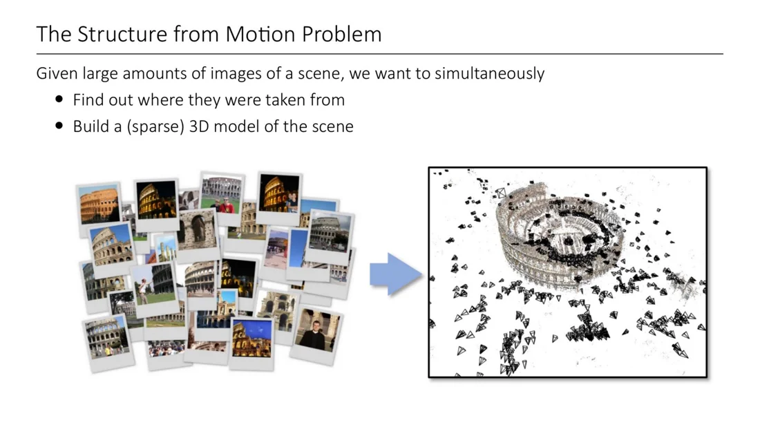
Photo Tourism (Snavely et al., SIGGRAPH 2006) was an early work on large photo collections: an interactive system to browse unstructured photo collections. It estimates camera poses and a sparse 3D reconstruction, so you can move smoothly between photographs.

Slide 6: Photo Tourism, reconstruction of the Trevi Fountain from 350 web photos (played 1.5x).

Over time the scale grew from single monuments to entire cities. Building Rome in a Day (Agarwal et al., ICCV 2009) reconstructs cities from web images (in 2009, Flickr had more than 2 million photos for “Rome”). “In a day” is the runtime of the whole pipeline. The scale brings new challenges:

• robustness: keypoint matching has no 3D awareness, so there will be outliers and mismatches
• large non-linear problems that need efficient algorithms (e.g. for bundle adjustment)
• parallel, distributed systems

Slide 7: Building Rome in a Day.

The SfM Problem

Slides 8-10

SfM problem

Given $m$ images of $n$ fixed 3D points such that

$$u_{ij}=P_i{X}_j$$

(in homogeneous coordinates), jointly estimate the camera matrices $P_i$ and the 3D points $X_j$.

• $u_{ij}$: projection of point $j$ onto image plane $i$ ($i$ = camera index, $j$ = point index)
• $P_i=K_i[R_i\mid t_i]$: intrinsics times global pose of camera $i$
• $X_j$: 3D point in world coordinates

We only know $u_{ij}$!

Slide 8: cameras and 3D points are both unknown.

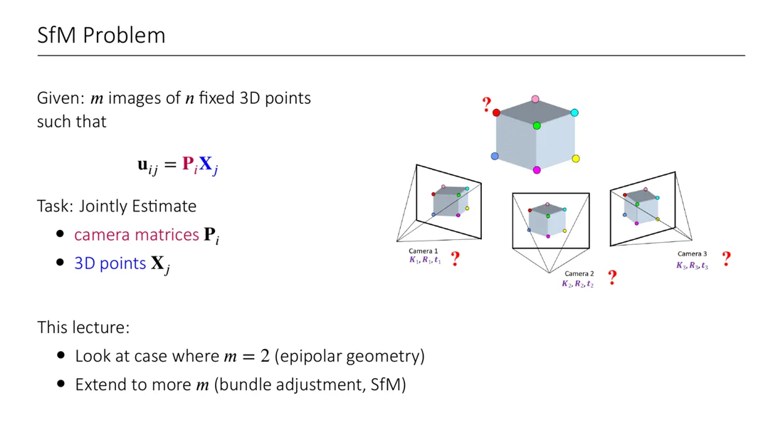
The lecture first looks at the case $m=2$ (epipolar geometry: how to estimate the relative orientation of two cameras), then extends to more images (bundle adjustment, SfM pipelines).

A note on correspondences

We assume we have precomputed 2D-2D correspondences: $u_{ij}\sim u_{i^{\prime }j}$ means both observe the point $X_j$ from cameras $i$ and $i^{\prime }$. They come from feature detection algorithms (SIFT, SURF, ORB, SuperPoint, …), which find keypoints, describe them by their surroundings, and match them between views. These methods are not part of this course. They are remarkably strong: SIFT can match the ground of Mars from two different views.

We do not assume the correspondences are correct. Dealing with outliers and wrong matches is a huge challenge in every SfM pipeline (→ RANSAC).

Three Components of SfM

Slides 11-13

The whole idea of SfM is to go from 2D-2D correspondences to camera poses and 3D points. Typically we first solve for motion, then infer the 3D points via triangulation.

flowchart LR
  C["Correspondences"] -- "SfM: estimate motion first" --> M["Camera poses<br/>(motion)"]
  M -- "triangulation" --> S["3D points<br/>(structure)"]
  S -- "pose estimation (PnP)" --> M

Problem	Given	Wanted
SfM	only 2D-2D correspondences	camera poses and 3D points
Triangulation	correspondences + known camera poses	3D points
Pose estimation (PnP)	2D-3D correspondences (3D points known)	camera pose

• Triangulation is a crucial part of most SfM pipelines, but a “simpler” problem, because the camera poses are already known.
• Pose estimation (Perspective-n-Point, PnP) is the inverse problem. It can be solved with the direct linear transform (see the exercise). It is an important step in incremental SfM: every new image has to be registered into the existing reconstruction.

Triangulation

Slides 14-16

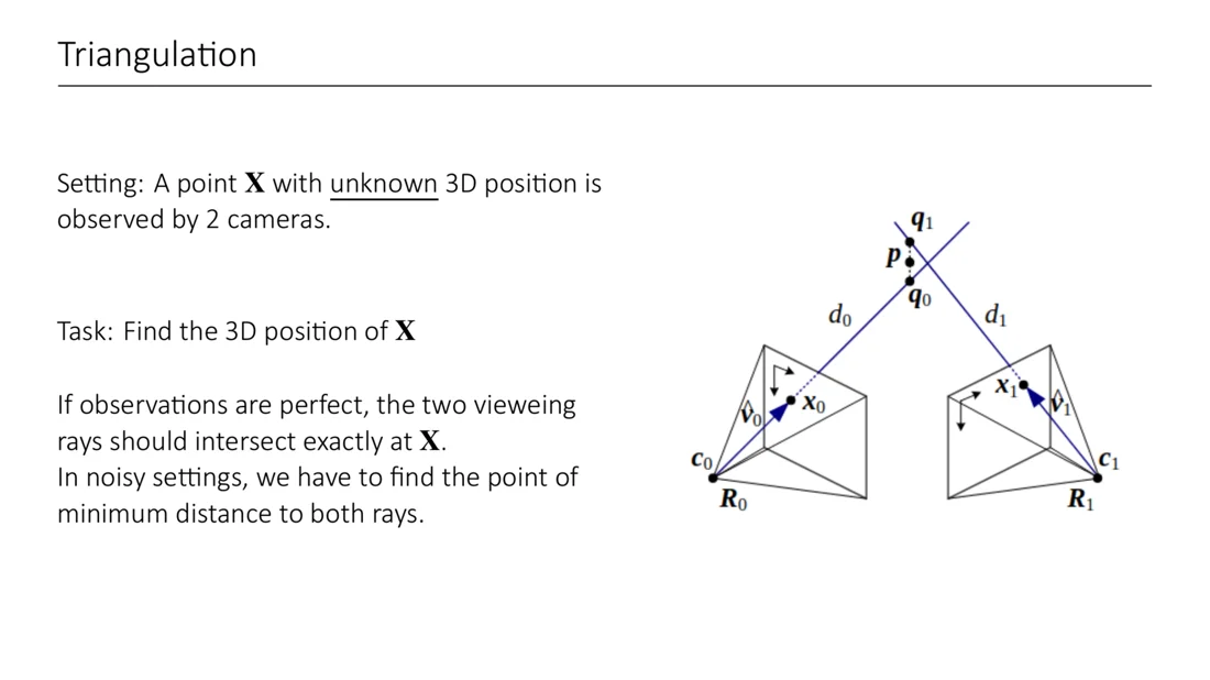
Setting: a point $X$ with unknown 3D position is observed by 2 cameras. Task: find the 3D position of $X$. With perfect observations, the two viewing rays intersect exactly at $X$. With noise, we look for the point with minimum distance to both rays.

Slide 14: with noise, the two rays don't intersect exactly.

Linear triangulation

The point is projected by the camera matrix, $u\simeq PX$ (equal up to scale). So $u$ and $PX$ are parallel, and their cross product is zero. This removes the unknown scale:

$$u\times PX=0⟺\left[\begin{array}{c}x\\ y\\ 1\end{array}\right]\times \left[\begin{array}{c}{P}_1^{T}X\\ P_2^{T}X\\ P_3^{T}X\end{array}\right]=0$$

where $P_k^T$ is the $k$-th row of $P$. The cross product evaluates to

$$\left[\begin{array}{c}y{P}_3^{T}X-P_2^{T}X\\ P_1^{T}X-x{P}_3^{T}X\\ x{P}_2^{T}X-y{P}_1^{T}X\end{array}\right]=0$$

The last row is a linear combination of the first two, so each camera gives 2 linear equations in $X$. One camera is not enough. With a second camera $P^{\prime }$ observing $u^{\prime }=(x^{\prime },y^{\prime })$, we stack:

Linear triangulation

$$\left[\begin{array}{c}y{P}_3^T-P_2^T\\ P_1^T-x{P}_3^T\\ y^{\prime }{P}_3^{\prime T}-P_2^{\prime T}\\ P_1^{\prime T}-x^{\prime }{P}_3^{\prime T}\end{array}\right]X=0$$

Solved in the least squares sense with SVD (the right singular vector of the smallest singular value, with $\Vert X\Vert =1$).

Epipolar Geometry

SfM usually estimates the motion (camera poses) from the 2D-2D correspondences first. We start with the simplest case: 2 cameras. First we need to understand the geometry of two such cameras.

Epipolar Plane, Baseline, Epipoles and Epipolar Lines

Slides 18-30

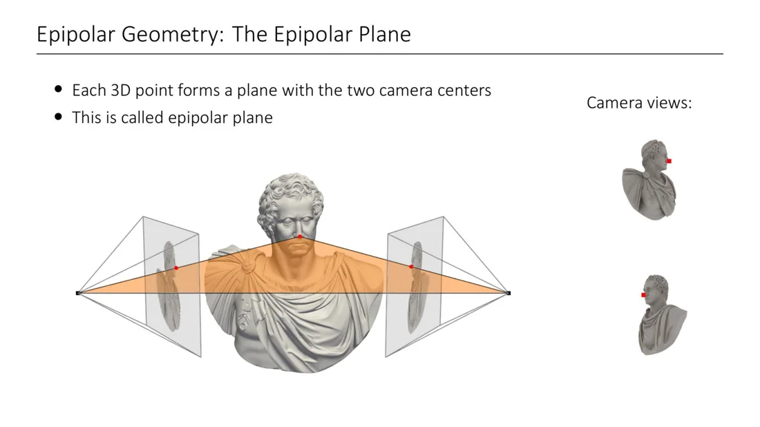
A scene is viewed by two cameras from slightly different angles.

Slide 20: the epipolar plane

Slide 23: baseline and epipoles

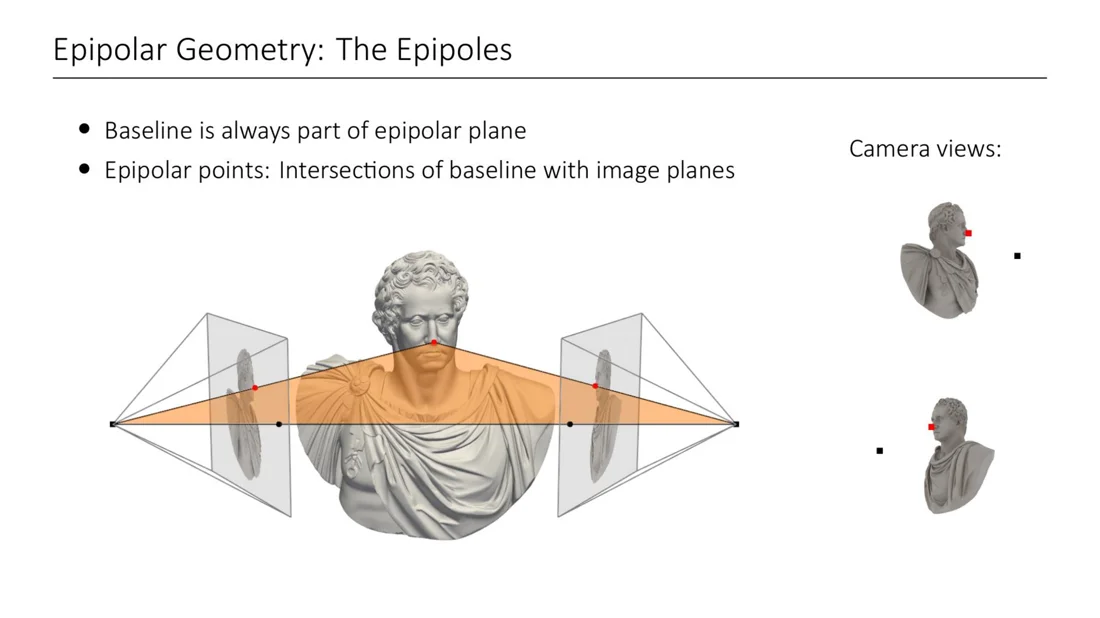
Epipolar geometry

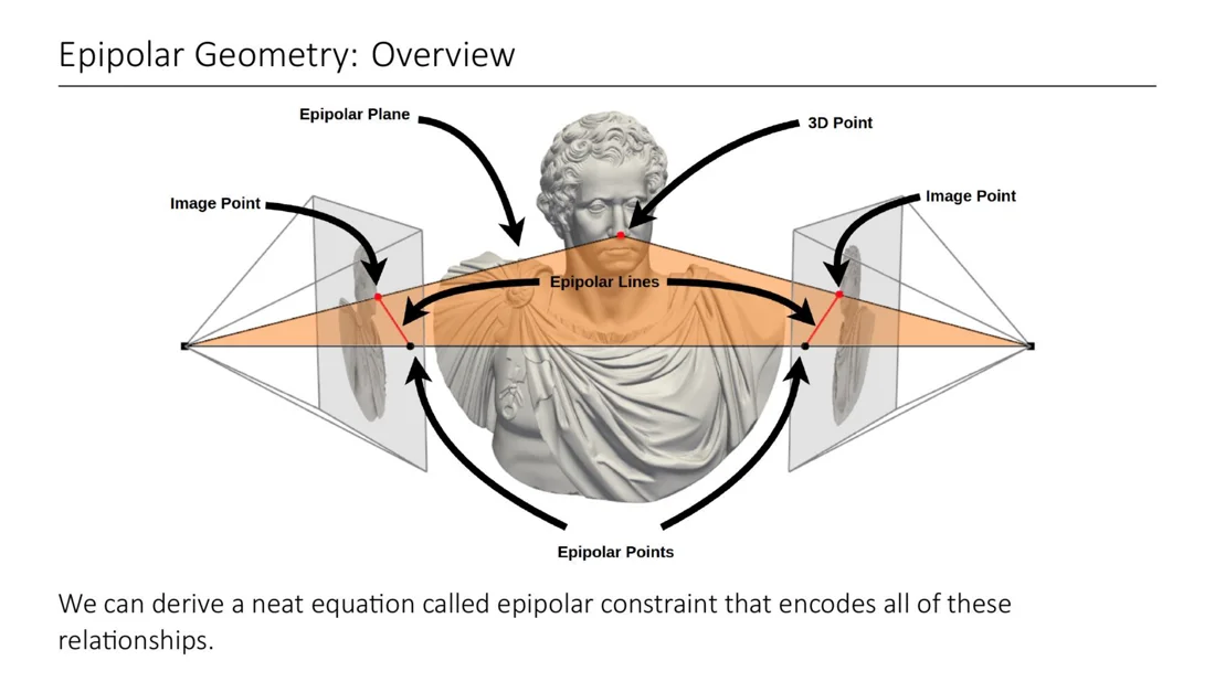
• Epipolar plane: every 3D point forms a plane with the two camera centers. It is different for every 3D point.
• Baseline: the line connecting the two camera centers. Since both centers are in every epipolar plane, the baseline is always part of it.
• Epipoles (epipolar points): the intersections of the baseline with the image planes. So they also lie in every epipolar plane.
• Epipolar lines: the intersections of the image planes with the epipolar plane. The epipolar line in image 1 is the projection of the viewing ray of camera 0 into image 1, and vice versa. It connects the observed point and the epipole.

The epipoles don’t have to lie inside the images: that depends on the relative orientation of the cameras, the focal lengths and the image size. If the cameras can’t see each other, the epipole is outside the image. It can even be at infinity.

When are the epipoles at infinity?

Answer

When the two viewing directions are parallel (the baseline is parallel to the image planes). Then the epipolar lines are parallel as well.

Slide 24: epipoles outside the images

Slide 25: epipolar lines

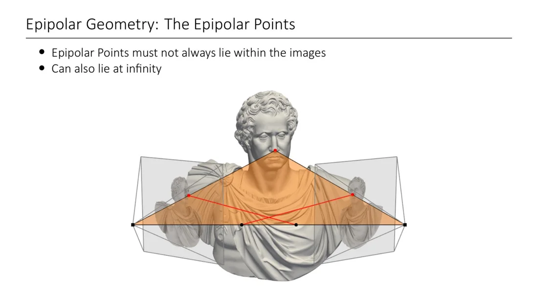
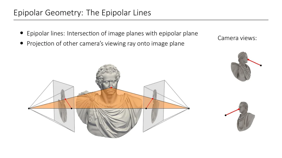
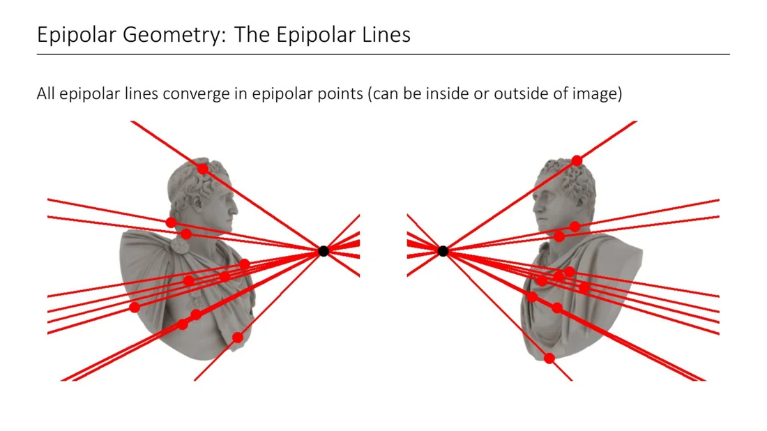
All epipolar lines in an image converge in the epipole (inside or outside the image).

Slide 26: all epipolar lines meet in the epipole.

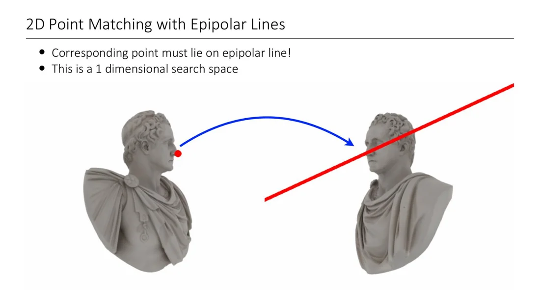
2D point matching with epipolar lines

Slides 28-29

Given 2 images and a point in one of them, find the matching point in the other. The naive approach searches the whole image (a 2D search space). With epipolar geometry we know the matching point must lie on the epipolar line (the projection of the viewing ray). This is a 1D search space. For this we need to know where the epipolar line is, which is what the math below gives us.

Slide 29: the match must lie on the epipolar line.

Overview (Slide 30)

3D point, image points, epipolar points and epipolar lines all lie on the epipolar plane. The epipolar constraint encodes all these relationships in one equation. From it we can later extract the relative camera poses.

Slide 30: epipolar geometry overview.

The Epipolar Constraint

Slides 31-33

Exam

This derivation is exactly what “understand the epipolar derivations” means. Be able to reproduce it step by step.

Formal setup

Slide 31

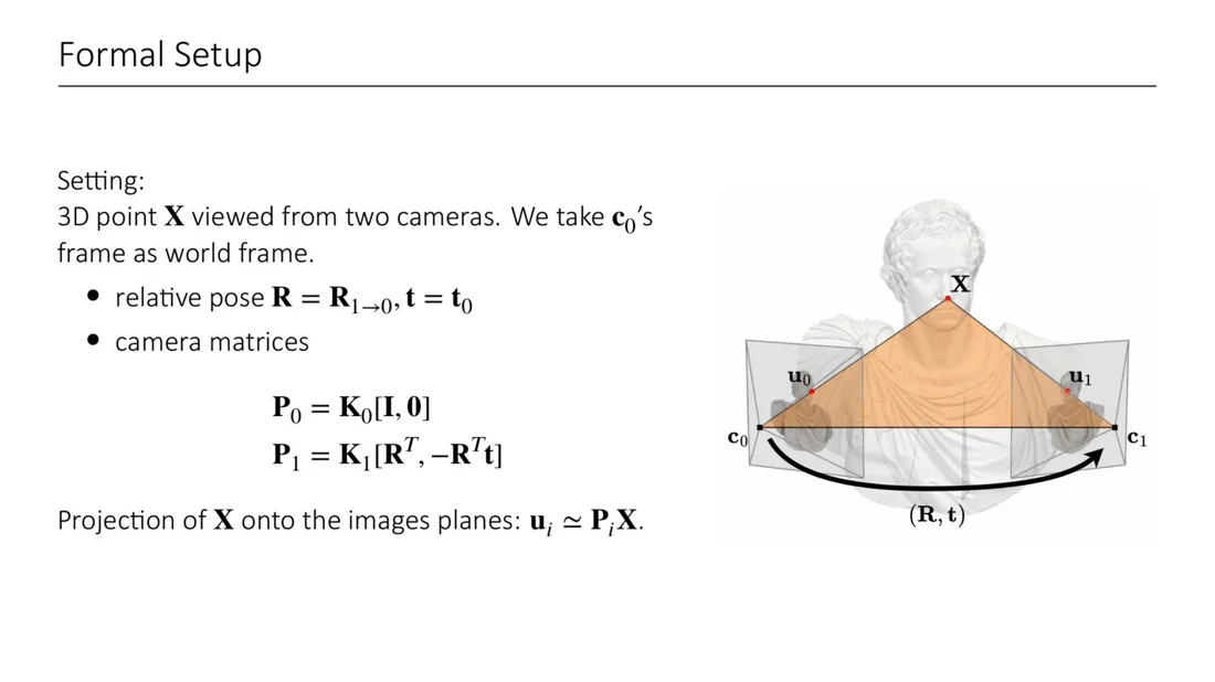
For now we assume we know everything about the cameras (intrinsics and extrinsics). Two cameras observe a single 3D point $X$. We don’t care about the “true” world frame, so we take camera 0’s frame as world frame.

Notation (important, other sources use other conventions)

• $R=R_{1\to 0}$: rotation from camera 1’s frame to camera 0’s frame
• $t=t_0$: camera 1’s center, expressed in camera 0’s frame
• Camera matrices:

$$P_0=K_0[I,0]P_1=K_1[R^T,-R^{T}t]$$

• Projection of $X$ onto the image planes: $u_i\simeq P_{i}X$

Slide 31: formal setup.

Derivation

Slides 32-33

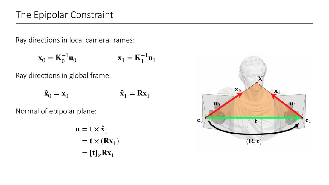
Step 1: ray directions in the local camera frames. $u_0,u_1$ are pixel coordinates, so we first compute the 3D ray directions by multiplying with the inverse calibration matrix:

$$x_0=K_0^{-1}{u}_0{x}_1=K_1^{-1}{u}_1$$

Step 2: ray directions in the global frame. Camera 0’s frame is the world frame, so $x_0$ is already global. Directions of camera 1 only have to be rotated:

$${\hat{x}}_0=x_0{\hat{x}}_1=R{x}_1$$

Step 3: normal of the epipolar plane. Two vectors in the plane are $t$ (the baseline, green in the figure) and ${\hat{x}}_1$ (the ray of camera 1, red). Their cross product is the normal. We write the cross product as a matrix product with the skew-symmetric matrix $[t{]}_{\times }$ (see hat operator):

$$n=t\times {\hat{x}}_1=t\times (R{x}_1)=[t{]}_{\times }R{x}_1$$

Step 4: $x_0$ lies in the epipolar plane too, so it is orthogonal to the normal: $⟨x_0,n⟩=0$.

Epipolar constraint and essential matrix

$$x_0^T[t{]}_{\times }R{x}_1=0⟺x_0^{T}E{x}_1=0,E:=[t{]}_{\times }R\in {\mathbb{R}}^{3\times 3}$$

Slide 32: t and R x₁ span the epipolar plane.

Intuition

Two image points that belong to the same 3D point must always satisfy this equation. The essential matrix captures the relative camera pose, $x_0$ and $x_1$ are the calibrated observations. The equation is just the coplanarity of the two rays and the baseline.

Essential Matrix

Slide 34

The essential matrix $E=[t{]}_{\times }R$ captures the epipolar geometry of the two cameras. It does not depend on the 3D point, only on the relative camera poses. From $E$ we can derive all the geometric relationships from before:

Properties of E (calibrated case)

• Epipoles: $E{\tilde{e}}_1=0={\tilde{e}}_0^{T}E$. The (calibrated) epipoles are the zero-value right and left singular vectors.
• Epipolar lines: ${\tilde{l}}_0=E{x}_1$ is the epipolar line corresponding to $x_1$ (in image 0), ${\tilde{l}}_1=E^T{x}_0$ is the epipolar line corresponding to $x_0$ (in image 1).
• $E$ has rank 2 and 5 degrees of freedom.

Why rank 2, and why 5 degrees of freedom?

Answer Rank 2: the epipoles are in the kernel of $E$. Or: $[t{]}_{\times }$ has rank 2 ($t$ is in its null space) and $R$ is invertible. 5 DoF: 3 for the rotation + 3 for the translation, minus 1 because $E$ is a projective mapping and only defined up to scale. You can scale $E$ and no equation changes.

All of these are in the calibrated (canonical camera) frame, because we used $x_i$ instead of $u_i$.

Fundamental Matrix

Slides 35-36

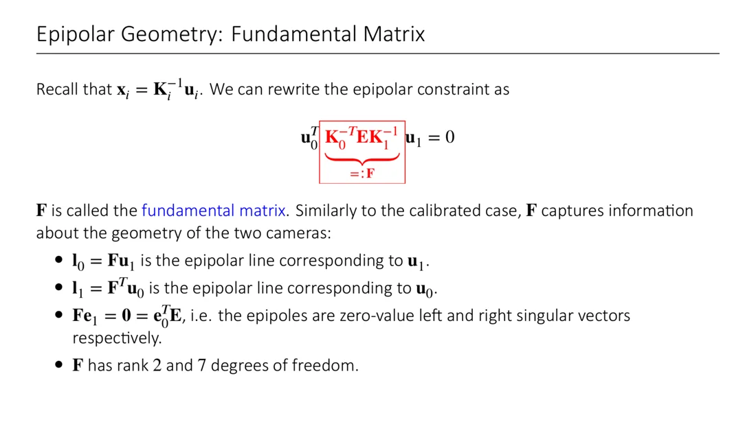
Going back to the uncalibrated case: with $x_i=K_i^{-1}{u}_i$ we rewrite the epipolar constraint in pixel coordinates:

Fundamental matrix

$$u_0^T\underset{=:F}{\underbrace{K_0^{-T}E{K}_1^{-1}}}{u}_1=0⟺u_0^{T}F{u}_1=0$$

($K_0^{-T}=(K_0^{-1}{)}^T=(K_0^T{)}^{-1}$, the order does not matter.)

$F$ captures the geometry of the two cameras in the same way:

• $l_0=F{u}_1$ is the epipolar line corresponding to $u_1$
• $l_1=F^T{u}_0$ is the epipolar line corresponding to $u_0$
• $F{e}_1=0=e_0^{T}F$: the epipoles are the zero-value right and left singular vectors
• $F$ has rank 2 (because $E$ has rank 2 and the $K_i$ have full rank) and 7 degrees of freedom: 9 entries, $-1$ for scale, $-1$ for $\det F=0$.

Why does the rank-2 constraint remove a degree of freedom for $F$ but not for $E$?

Answer $F$ starts from an arbitrary $3\times 3$ matrix, so $\det F=0$ is a new constraint. $E$ is built from $R$ and $t$, and its rank 2 already follows from $[t{]}_{\times }$ having rank 2. There is no new constraint.

	Essential matrix $E$	Fundamental matrix $F$
Constraint	$x_0^{T}E{x}_1=0$	$u_0^{T}F{u}_1=0$
Coordinates	calibrated rays $x_i=K_i^{-1}{u}_i$	pixels $u_i$
Definition	$E=[t{]}_{\times }R$	$F=K_0^{-T}E{K}_1^{-1}$
Needs intrinsics?	yes	no
Rank / DoF	2 / 5	2 / 7

Summary: epipolar constraint (Slide 36)

Each correspondence pair $u_0,u_1$ must satisfy $u_0^{T}F{u}_1=0$. It is expressed with $F$ (uncalibrated) or $E$ (calibrated). If we know $F$ or $E$, we can derive a lot: epipoles, epipolar lines, and the relative pose.

Slide 35: the fundamental matrix.

Recovering the Relative Pose from E

Slides 37-40

We want the relative camera pose from 2D-2D correspondences, and $E=[t{]}_{\times }R$ is a product of $t$ and $R$. Can we decompose $E$ into $t$ and $R$? Yes, up to scale, with a decomposition theorem (Hartley & Zisserman, 9.6).

Decomposition of E

The SVD of an essential matrix has the form (up to scale)

$$E=U\text{diag}(1,1,0)V^T,U=[u_1{u}_2{u}_3],V^T=\underset{W}{\underbrace{\left[\begin{array}{ccc}0& -1& 0\\ 1& 0& 0\\ 0& 0& 1\end{array}\right]}}{U}^{T}R$$

So we recover $R$ and $t$ (up to scale) as

$$t=u_3\text{ or }-u_{3}R=UW{V}^T\text{ or }U{W}^T{V}^T$$

Why $t=\pm u_3$

$t\times t=0$, so $[t{]}_{\times }t=0$ and $t^{T}E=t^T[t{]}_{\times }R=0$: $t$ is in the left null space of $E$, i.e. the singular vector $u_3$ with singular value 0. The sign and the length can’t be determined.

This gives 4 possible solutions for the relative orientation of the two cameras.

Slide 39: the four solutions (Hartley & Zisserman, Fig. 9.12). Only in (a) the point is in front of both cameras.

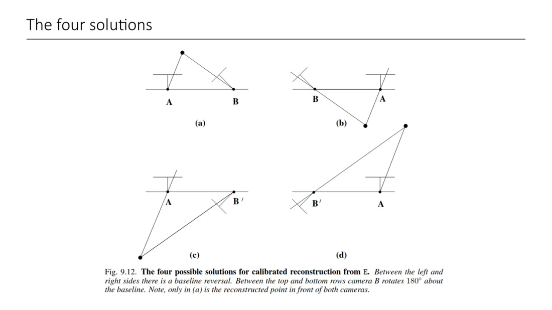
How do we find the correct one? Triangulate a single correspondence and check that the point is in front of both cameras (positive depth). Only one of the four configurations passes.

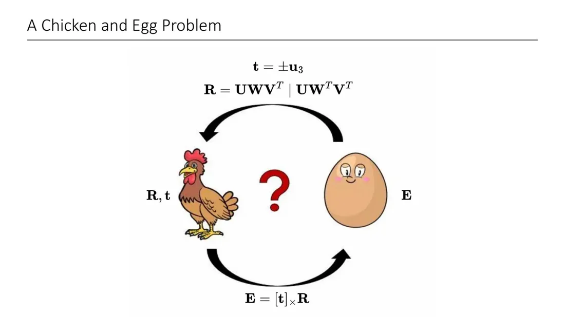
A chicken and egg problem

Slide 40

• Given the relative pose, we can compute $E=[t{]}_{\times }R$.
• Given $E$, we can recover $t$ and $R$ (up to scale).

But how do we get $E$ without knowing $t$ and $R$? Next: estimate $E$ (or $F$) from 2D-2D correspondences alone.

Slide 40: the chicken and egg problem.

Estimating the Fundamental / Essential Matrix

So far we derived formulas for $E$, $F$ and the epipolar constraint, assuming known relative poses. Now the relative poses are unknown: given a set of correspondences, we want to extract them. For this we estimate $F$ or $E$ from the correspondences.

One Equation per Correspondence

Slides 43-44

A correspondence pair $u_0=(x_0,y_0,1)$, $u_1=(x_1,y_1,1)$ must satisfy $u_0^{T}F{u}_1=0$. Written out, this is linear in the 9 entries of $F$:

$$x_0{f}_{11}{x}_1+x_0{f}_{12}{y}_1+x_0{f}_{13}+y_0{f}_{21}{x}_1+y_0{f}_{22}{y}_1+y_0{f}_{23}+f_{31}{x}_1+f_{32}{y}_1+f_{33}=0$$

How many correspondences do we need to estimate F?

Answer

• For the fundamental matrix, 8 points suffice → 8-point algorithm (9 entries, minus scale).
• $F$ has 7 degrees of freedom, so even 7 points suffice, but then the problem is no longer linear (the determinant constraint is non-linear) → 7-point algorithm.
• For the essential matrix, even 5 points are enough → 5-point algorithm.

The 8-Point Algorithm

Slides 45-49

Given $M$ correspondences ($M=8$, but more is better), stack the $M$ linear equations. Row $j$ is built from the $j$-th correspondence:

$$\underset{W\in {\mathbb{R}}^{M\times 9}}{\underbrace{\left[\begin{array}{ccccccccc}{x}_{1,0}{x}_{1,1}& x_{1,0}{y}_{1,1}& x_{1,0}& y_{1,0}{x}_{1,1}& y_{1,0}{y}_{1,1}& y_{1,0}& x_{1,1}& y_{1,1}& 1\\ ⋮& & & & & & & & ⋮\\ x_{M,0}{x}_{M,1}& x_{M,0}{y}_{M,1}& x_{M,0}& y_{M,0}{x}_{M,1}& y_{M,0}{y}_{M,1}& y_{M,0}& x_{M,1}& y_{M,1}& 1\end{array}\right]}}\left[\begin{array}{c}{f}_{11}\\ ⋮\\ f_{33}\end{array}\right]=Wf=0$$

In practice we use $M>8$ correspondences to reduce the effect of noisy measurements. Then there is no exact solution, and we solve in the least squares sense:

Least squares with SVD

$$\underset{\Vert f\Vert =1}{\min }\Vert Wf{\Vert }_2^2,W=U\Sigma V^T$$

The least squares solution is the right singular vector corresponding to the smallest singular value (last column of $V$). We get the estimate $\hat{F}$ by reshaping $f$ into $3\times 3$. The constraint $\Vert f\Vert =1$ excludes $f=0$ and fixes the free scale.

Problem: rank

Slide 47: estimate with full rank, lines don't meet

Slide 49: after enforcing rank 2

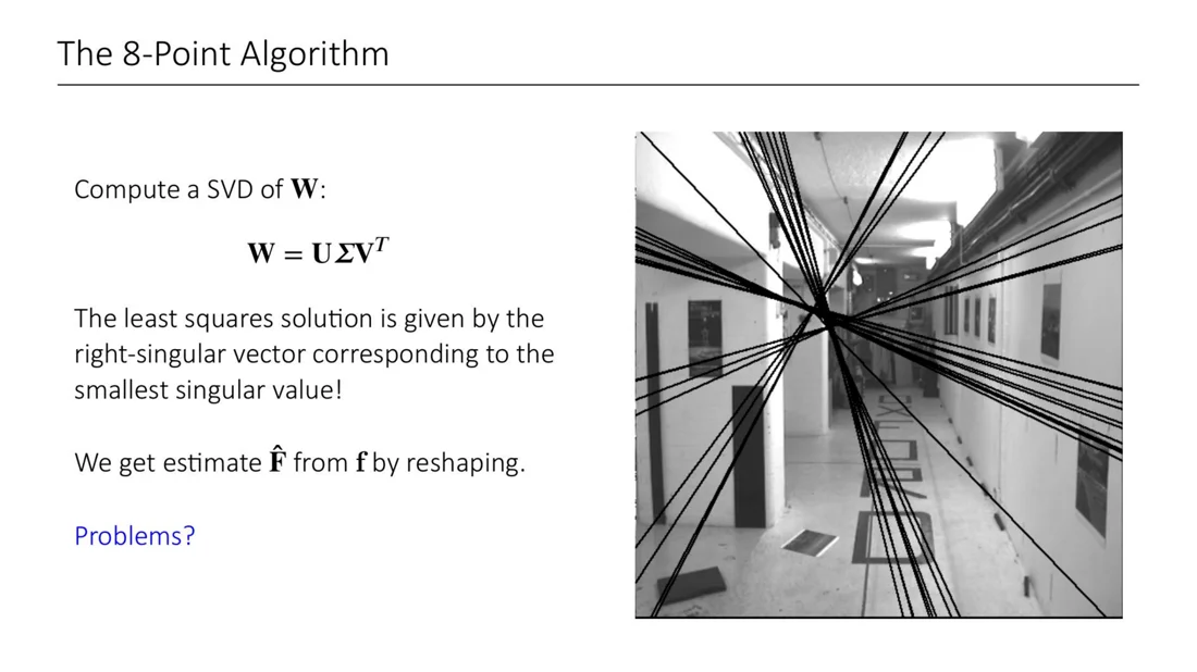
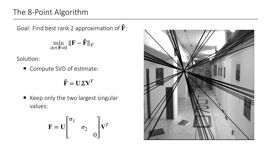
The epipolar lines from this estimate don’t converge in a single epipole. The reason: with noise, $\hat{F}$ has full rank, but an essential / fundamental matrix has rank 2 (the epipoles are its null vectors).

Enforce rank 2

Find the best rank-2 approximation of $\hat{F}$:

$$\underset{\det F=0}{\min }\Vert F-\hat{F}{\Vert }_F$$

Solution: compute another SVD $\hat{F}=U\Sigma V^T$ and keep only the two largest singular values:

$$F=U\left[\begin{array}{ccc}{\sigma }_1& & \\ & {\sigma }_2& \\ & & 0\end{array}\right]V^T$$

Normalization: the Normalized 8-Point Algorithm

Slides 50-53

One row of $W$ is $[x_{1,0}{x}_{1,1},x_{1,0}{y}_{1,1},x_{1,0},\dots ,1]$. Typically $x,y\in [0,2000]$, so:

• the entries differ by orders of magnitude (about $10^6$ vs. $1$)
• $W$ is highly unbalanced and not well conditioned
• this creates problems during the SVD

Solution: transform the image coordinates so that $W$ becomes better conditioned. For each image $i$, apply a transformation $T_i$:

• translate the image points so that their centroid is at the origin
• uniformly scale them so that the mean squared distance of the points from the origin is about 2 px

Slide 52: normalization with T.

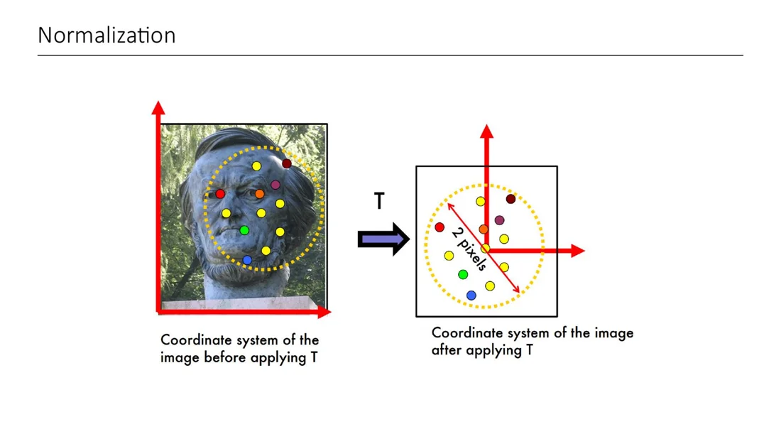
Normalized coordinates

New homogeneous coordinates ${\bar{x}}_i=T_i{x}_i$. The epipolar constraint becomes

$$0={\bar{x}}_0^T{T}_0^{-T}F{T}_1^{-1}{\bar{x}}_1={\bar{x}}_0^T\bar{F}{\bar{x}}_1,\bar{F}=T_0^{-T}F{T}_1^{-1}$$

So we estimate $\bar{F}$ with the 8-point algorithm and recover

$$F=T_0^T\bar{F}{T}_1$$

The 8-point algorithm: summary (Slide 53)

1. Normalize points
2. Construct the $M\times 9$ matrix $W$
3. Find the SVD of $W=U\Sigma V^T$
4. The entries of $\hat{F}$ are the elements of the column of $V$ corresponding to the smallest singular value
5. Find the SVD of $\hat{F}=U^{\prime }{\Sigma }^{\prime }{V}^{\prime T}$
6. Set $F=U^{\prime }\text{diag}({\sigma }_1^{\prime },{\sigma }_2^{\prime },0)V^{\prime T}$
7. Denormalize $F$

Exam

Know the algorithm step by step and when it is used: whenever $F$ is estimated linearly from pixel correspondences, e.g. inside RANSAC for the geometric verification and for the initialization of an SfM pipeline. With known intrinsics, the 5-point algorithm for $E$ is preferred.

RANSAC: Robustness to Outliers

Slides 54-57

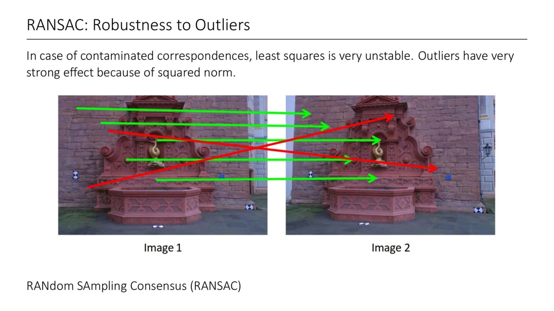
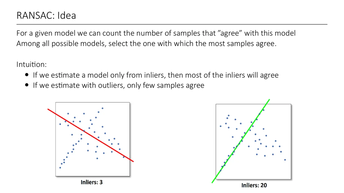
A very important theme in reconstruction from 2D correspondences is robustness to wrong correspondences: some points are matched to false points because they locally look similar. With contaminated correspondences, least squares is very unstable: outliers have a very strong effect because of the squared norm.

Slide 54: correct matches (green) and outliers (red).

Line fitting example: fit a line to 2D points. The least squares fit is pulled away by the outliers (squared distances punish large deviations even more). The intuitively “best” line is the one with the most inliers.

Slide 55: least squares fit

Slide 56: 3 inliers vs. 20 inliers

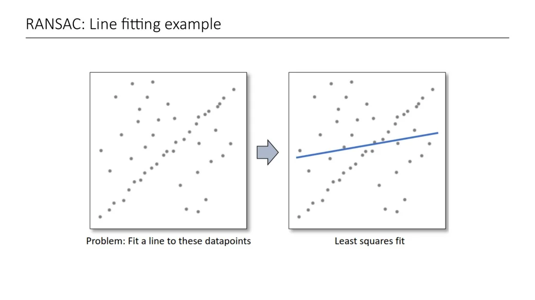
RANSAC (RANdom SAmple Consensus): idea

For a given model, count the number of samples that agree with it. Among all possible models, select the one with which the most samples agree.

• If we estimate a model only from inliers, most of the inliers will agree.
• If we estimate it with outliers, only few samples agree.

RANSAC algorithm

1. Randomly choose $s$ samples. Typically $s$ = the minimal sample size to fit a model (line fitting: 2, essential matrix: 5, fundamental matrix: 8).
2. Fit a model to those samples.
3. Count the number of inliers.
4. Update the best solution found so far.
5. Repeat.

How many iterations? With an outlier ratio $e$ and a desired probability $p$ of getting a correct solution:

$$N\ge \frac{\log (1-p)}{\log \left(1-(1-e{)}^s\right)}$$

Intuition

$(1-e{)}^s$ is the probability that one random sample has only inliers. Smaller samples and fewer outliers need fewer iterations. That is why minimal solvers (like the 5-point algorithm) are preferred inside RANSAC.

From Fundamental to Essential Matrix

Slide 58

Now we have a robust way to compute $F$ with the 8-point algorithm. If we can recover the intrinsic matrices $K_0,K_1$ (they often come as part of the image metadata), we get the essential matrix from $F=K_0^{-T}E{K}_1^{-1}$, i.e. $E=K_0^{T}F{K}_1$.

An ideal essential matrix has two identical singular values, up to scale $E=U\text{diag}(1,1,0)V^T$. So we project the estimated $E$ such that the singular values are $1,1,0$.

Relative pose from 2D-2D correspondences: the full pipeline

flowchart LR
  A["2D-2D<br/>correspondences"] --> B["F: normalized<br/>8-point + RANSAC"]
  B --> C["E = K0ᵀ F K1<br/>singular values 1, 1, 0"]
  C --> D["SVD of E:<br/>4 candidates for R, t"]
  D --> E2["point in front of<br/>both cameras"]
  E2 --> F2["triangulate<br/>3D points"]

$t$ is only known up to scale.

Bundle Adjustment and SfM

From Two Views to N Views

Slide 60

So far: epipolar geometry takes us from correspondences on two images to the relative camera poses (8-point algorithm) and the 3D points (triangulation). Extensions to 3 or 4 views exist (trifocal, quadrifocal tensors), but get complicated. Instead, most SfM pipelines incrementally add images to a model and update it with every new observation. The key ingredient is bundle adjustment, which optimizes the registered camera poses and 3D points together.

Bundle Adjustment

Slides 61-62

Bundle adjustment

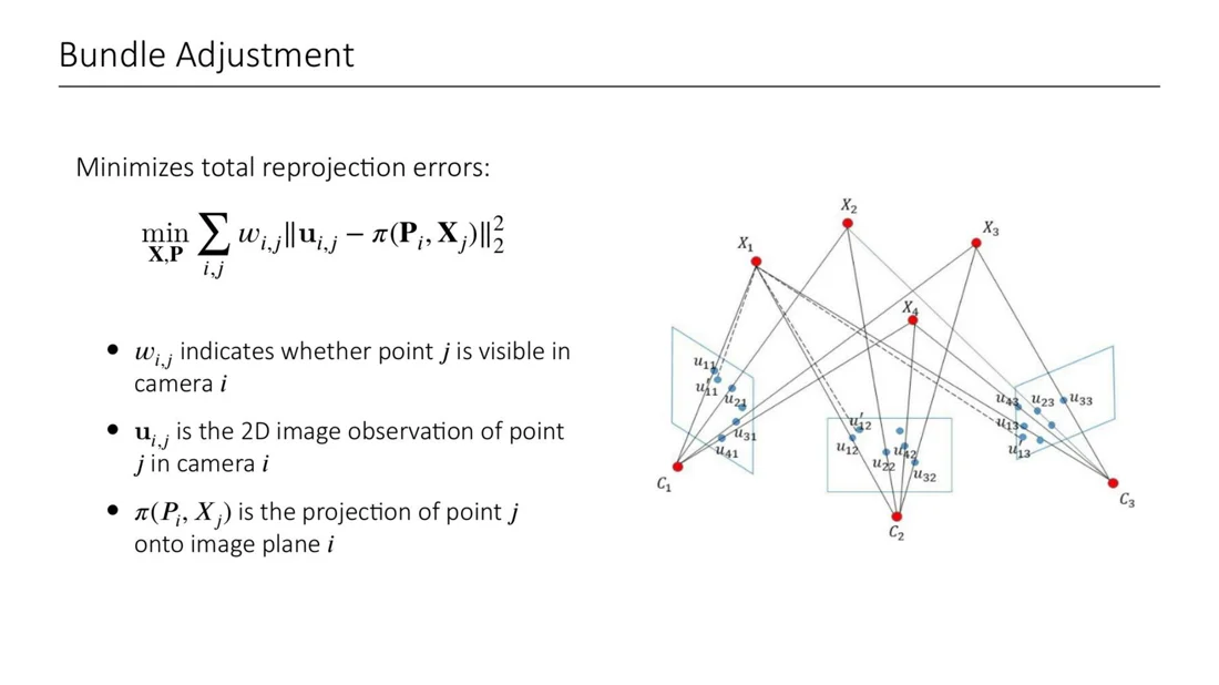
Minimize the total reprojection error over all 3D points $X$ and camera matrices $P$:

$$\underset{X,P}{\min }\sum _{i,j}{w}_{i,j}{\Vert u_{i,j}-\pi (P_i,X_j)\Vert }_2^2$$

• $w_{i,j}$: indicator whether point $j$ is visible in camera $i$
• $u_{i,j}$: the actual 2D observation of point $j$ in camera $i$
• $\pi (P_i,X_j)$: the projection of point $j$ onto image plane $i$ with the current estimates

Slide 61: every visible point-camera pair contributes a reprojection error.

Reprojection error

“How far is the reprojection with the current estimates from the actual observation?” Only point-camera pairs that are actually visible count.

Why can’t we just solve SfM with bundle adjustment?

• It is usually solved with Gauss-Newton or Levenberg-Marquardt. For large systems, efficient open source tools exist (e.g. Google Ceres), and they can use the sparse structure of the problem. It is still time consuming.
• Exact methods have cubic runtime (in the number of cameras), approximate methods linear runtime. For whole cities this is not feasible.
• It is sensitive to initialization and only finds local minima.

Therefore, bundle adjustment is only used as a refinement step in SfM pipelines, after epipolar geometry and triangulation. Some variants optimize only the cameras (points fixed) or only the points to save time.

3D Reconstruction Pipeline

Slides 63-65

flowchart LR
  A["Unstructured<br/>images"] -- "data association" --> B["Scene graph"]
  B -- "SfM" --> C["Sparse model<br/>(poses + sparse points)"]
  C -- "MVS" --> D["Dense model"]

Slide 63: the 3D reconstruction pipeline. Dense reconstruction (MVS) is part of Lecture 4.

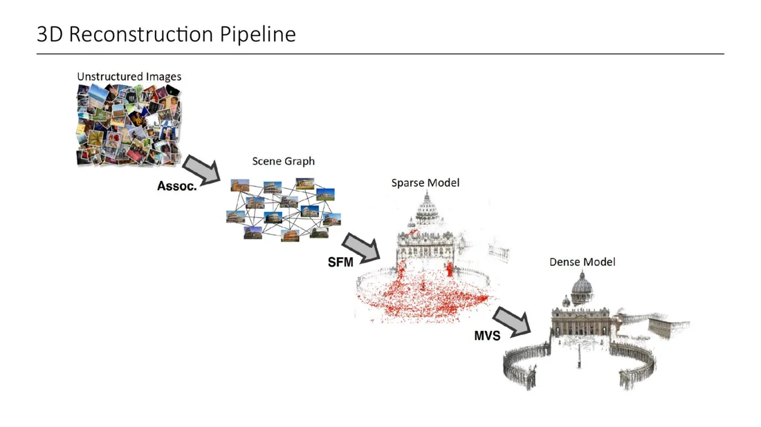
The dense step (MVS) is explained in Lecture 4.

Data association

Slide 64

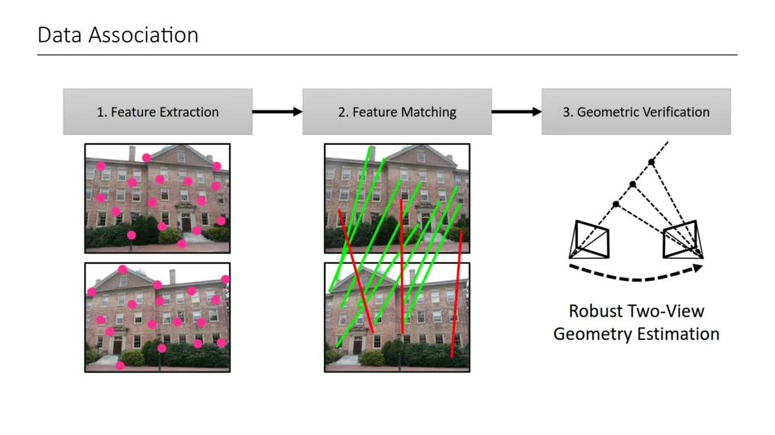
1. Feature extraction: identify keypoints and extract local features (e.g. SIFT).
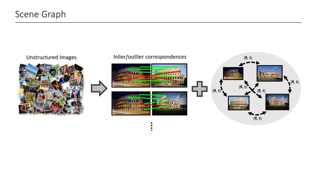
2. Feature matching: match features between images to get 2D-2D correspondences. The naive way compares every feature with every feature in every other image; there are more scalable approaches.
3. Geometric verification: the matching is based on appearance only, without spatial reasoning, so many matches are wrong. We robustly estimate the two-view geometry with epipolar geometry (essential matrix + relative pose, with RANSAC). If enough matches are geometrically consistent, the two views are “geometrically verified” and connected by an edge in the scene graph.

Slide 64: data association.

Scene graph

Slide 65

After data association we have the scene graph: nodes are images, edges are geometrically verified image pairs with their inlier correspondences and first estimates of the relative poses $(R,t)$. It tells us (somewhat reliably) which images overlap.

Slide 65: the scene graph.

Structure from Motion Paradigms

Slide 66

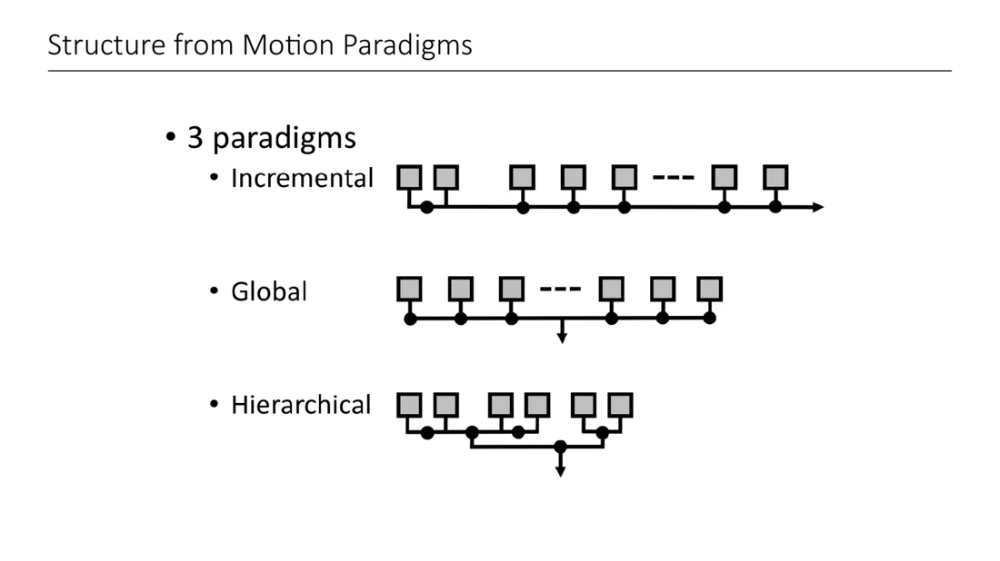
Most SfM pipelines fall into one of three categories:

• Incremental: start from two views, and add one more view in each step.
• Global: process all views simultaneously.
• Hierarchical: a mix of both. Partition the scene graph into clusters, reconstruct them individually, then stitch them together.

Slide 66: the three SfM paradigms.

Incremental SfM (COLMAP)

Slides 67-75

COLMAP is the most popular incremental SfM pipeline. You can see that it is incremental: it adds one camera after the other, together with the newly observed 3D points.

Slide 67: COLMAP reconstruction of 66 images (played 3x).

Slide 68: COLMAP method overview. Correspondence search (feature extraction, matching, geometric verification) and incremental reconstruction (initialization, image registration, triangulation, bundle adjustment, outlier filtering).

Incremental SfM

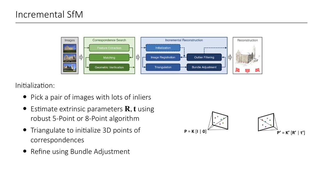
Initialization:

1. Pick a pair of images with lots of inliers.
2. Estimate the extrinsic parameters $R,t$ with the robust 5-point or 8-point algorithm. The first camera is $P=K[I\mid 0]$, the second $P^{\prime }=K^{\prime }[R^{\prime }\mid t^{\prime }]$.
3. Triangulate to initialize the 3D points of the correspondences.
4. Refine using bundle adjustment.

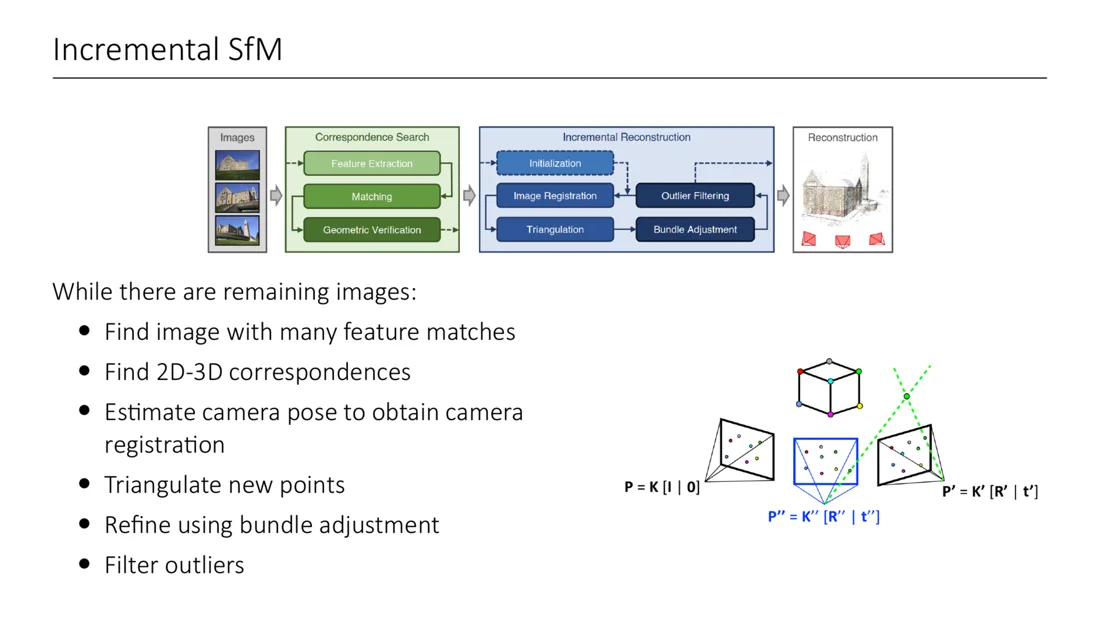
While there are remaining images:

1. Find the image with many feature matches.
2. Find 2D-3D correspondences (to the existing 3D points).
3. Estimate the camera pose (PnP) to obtain the camera registration $P^{\prime \prime }=K^{\prime \prime }[R^{\prime \prime }\mid t^{\prime \prime }]$.
4. Triangulate new points.
5. Refine using bundle adjustment.
6. Filter outliers.

Slide 74: a new camera is registered via 2D-3D correspondences.

Incremental SfM: challenges (Slide 75)

The initial pair must be chosen carefully:

• a bad choice leads to an unrecoverable local minimum
• the cameras should be far apart for a robust initialization
• dense feature regions are more robust because of redundancies, but bundle adjustment is slower

Next best view problem:

• an almost identical view → high uncertainty in triangulation
• a very different view → low overlap and high camera uncertainty
• a single bad choice may impact the whole reconstruction

Global SfM (GLOMAP)

Slides 76-80

Don’t add views incrementally. Solve for all global poses in one pass. In the GLOMAP demo, all cameras and points are optimized simultaneously.

Slide 76: GLOMAP, global SfM (ECCV 2024).

Given the relative rotation and translation estimates, can we recover the global rotations and translations of the cameras? From pairwise two-view geometry we get relative poses $\{R,t{\}}_{ij}$ between all cameras that see a common region. They form a view graph. These estimates are noisy (wrong correspondences, inaccurate intrinsics), so we can’t simply chain them: every cycle in the view graph can lead to a clash in the global poses. This is solved with rotation and translation averaging.

Slide 77: the view graph.

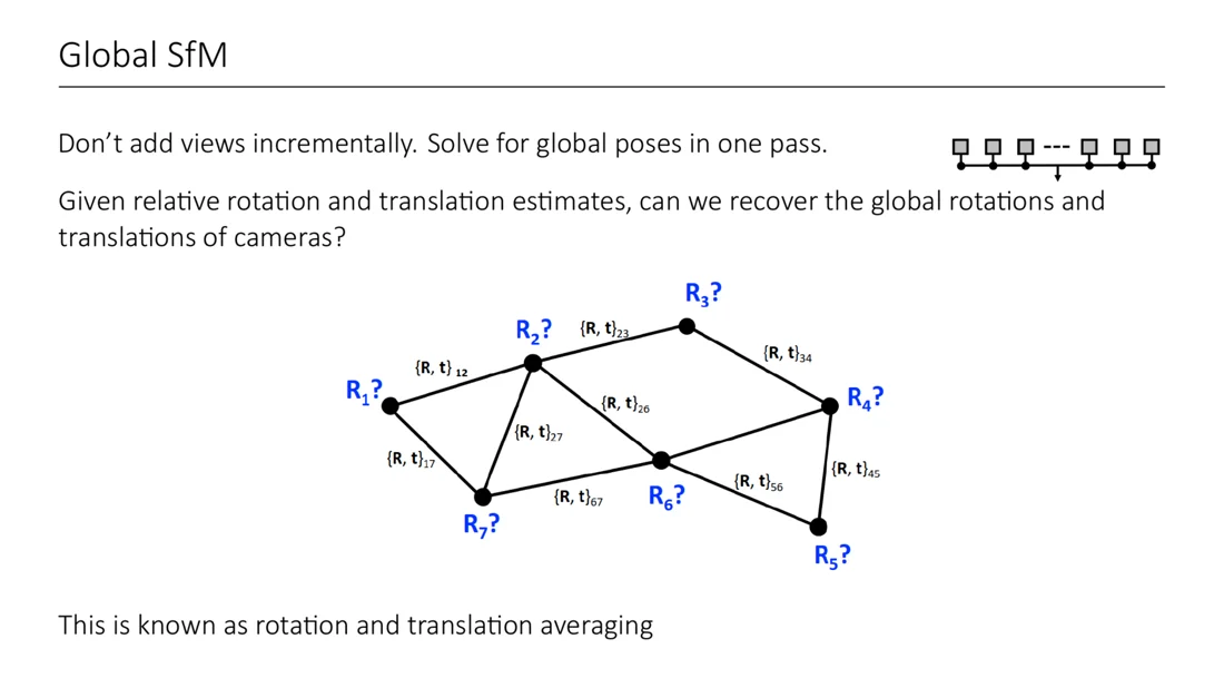
Rotation averaging

Estimate the global rotations that minimize the relative rotation error:

$$\underset{\hat{R}}{\min }\Vert R_{ij}-{\hat{R}}_j{\hat{R}}_i^T\Vert$$

$\hat{R}=[{\hat{R}}_1,\dots ,{\hat{R}}_N]$ are the global camera rotations we optimize for, $R_{ij}$ is the relative rotation estimate between cameras $i$ and $j$ (from epipolar geometry). In global rotations, the relative rotation is ${\hat{R}}_j{\hat{R}}_i^T$ (“back and forth”).

Translation averaging

Similarly, estimate (and filter) the global translations:

$$\underset{\hat{t}}{\min }\Vert t_{ij}-\frac{{\hat{t}}_i-{\hat{t}}_j}{\Vert {\hat{t}}_i-{\hat{t}}_j\Vert }\Vert$$

The distances are normalized because we can only recover the $t_{ij}$ up to scale.

GLOMAP (Fan et al., ECCV 2024) revisits global SfM after years of COLMAP. There is no loop in the pipeline (no incremental view adding): a global estimation followed by bundle adjustment. It is up to 1-2 orders of magnitude faster than COLMAP with similar or better quality. GLOMAP does not do translation averaging: it introduces global positioning, which estimates the camera translations and the 3D points together (instead of translation averaging followed by triangulation).

Slide 80: the GLOMAP pipeline (rotation averaging, global positioning, bundle adjustment, structure refinement).

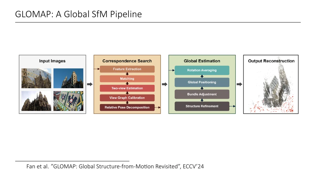
Hierarchical SfM and Comparison

Slides 81-82

Hierarchical SfM:

1. Hierarchically cluster the scene graph.
2. Reconstruct each cluster independently.
3. Merge the clusters using similarity transformations (each cluster has its own frame and scale).

Method	Efficiency	Robustness	Accuracy	Examples
Incremental	−	++	+	OpenSfM, COLMAP
Global	+	+	+	OpenMVG, Theia, GLOMAP
Hierarchical	++	−	−

Teaser: learning-based methods are taking over (→ Lecture 9).

Challenges

Slides 83-89

• WTFs (watermarks, timestamps, frames): they create matches at the image border that are geometrically consistent (a pure translation), but wrong. Detect translations at the image border.
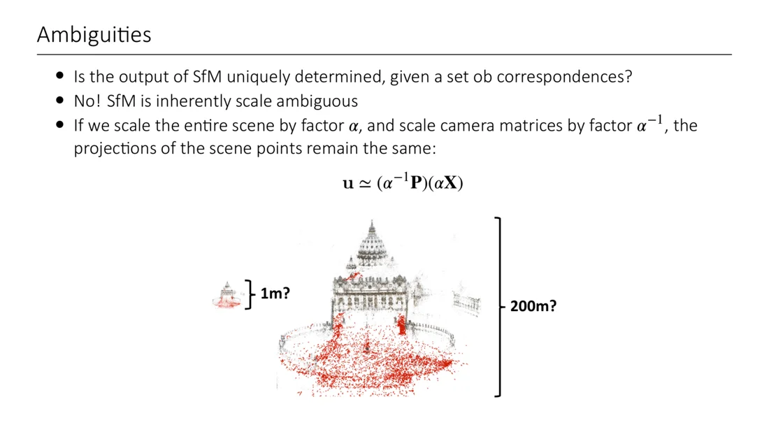
• Ambiguities: is the output of SfM uniquely determined by the correspondences? No, SfM is inherently scale ambiguous. Scaling the scene by $\alpha$ and the camera matrices by ${\alpha }^{-1}$ gives the same projections:

$$u\simeq ({\alpha }^{-1}P)(\alpha X)$$

Is the reconstruction 1 m or 200 m large? The images can’t tell.

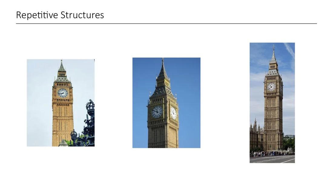
• Repetitive structures: e.g. the four identical faces of Big Ben. Matches between different faces look consistent but are wrong.
• Dynamic scenes: moving objects (people, cars) violate the assumption of a static scene.
• Illumination / weather change: day and night photos of the same place are hard to match.

Slide 86: scale ambiguity

Slide 87: repetitive structures

Worked Example: RANSAC Iterations

How many RANSAC iterations for the fundamental matrix?

Assume 50% outliers ($e=0.5$), the 8-point algorithm ($s=8$) and a desired success probability $p=0.99$:

$$N\ge \frac{\log (1-0.99)}{\log \left(1-0.5^8\right)}=\frac{\log 0.01}{\log (1-0.00390625)}\approx \frac{-4.605}{-0.003914}\approx 1177$$

With the 5-point algorithm for $E$ ($s=5$): $N\ge \frac{\log 0.01}{\log (1-0.5^5)}=\frac{-4.605}{-0.03175}\approx 146$. This is why minimal solvers are preferred inside RANSAC.

Summary

The SfM pipeline in one picture

flowchart TD
  I["Images"] --> F1["Feature extraction (SIFT)"] --> F2["Feature matching"]
  F2 --> GV["Geometric verification:<br/>F or E with RANSAC"]
  GV --> SG["Scene graph"]
  SG --> INIT["Initial pair: R, t from E<br/>triangulate, bundle adjustment"]
  INIT --> LOOP["Next image: 2D-3D matches, PnP,<br/>triangulate, bundle adjustment, filter"]
  LOOP --> LOOP
  LOOP --> SP["Sparse model"] --> MVS["MVS: dense model"]

Self-Test

What is the SfM problem, and how do triangulation and PnP relate to it?

Answer $u_{ij}=P_i{X}_j$, only $u_{ij}$ known). Triangulation: poses known → 3D points. PnP: 2D-3D correspondences → camera pose. SfM usually first estimates the motion, then triangulates.

From 2D correspondences only, jointly estimate the camera matrices and sparse 3D points (

How does linear triangulation work?

Answer $u\simeq PX$, so $u\times PX=0$. Each camera gives 2 independent linear equations in $X$. Stack the equations of both cameras into $AX=0$ and solve with SVD (right singular vector of the smallest singular value).

Define epipolar plane, baseline, epipole and epipolar line.

Answer

Epipolar plane: spanned by the 3D point and both camera centers. Baseline: the line between the camera centers, part of every epipolar plane. Epipole: intersection of the baseline with an image plane. Epipolar line: intersection of the epipolar plane with an image plane, i.e. the projection of the other camera’s viewing ray. All epipolar lines go through the epipole.

Why do epipolar lines help with matching?

Answer

The corresponding point must lie on the epipolar line, so the search is 1D instead of 2D.

Derive the epipolar constraint.

Answer $x_i=K_i^{-1}{u}_i$. In camera 0's frame the rays are $x_0$ and $R{x}_1$. The baseline $t$ and $R{x}_1$ span the epipolar plane, so its normal is $n=t\times R{x}_1=[t{]}_{\times }R{x}_1$. $x_0$ also lies in the plane: $x_0^T[t{]}_{\times }R{x}_1=0$, i.e. $x_0^{T}E{x}_1=0$ with $E=[t{]}_{\times }R$.

Calibrated rays

Essential vs. fundamental matrix: definition, rank, degrees of freedom?

Answer $E=[t{]}_{\times }R$ works on calibrated rays and needs the intrinsics: rank 2, 5 DoF (3 + 3 − 1 for scale). $F=K_0^{-T}E{K}_1^{-1}$ works on pixels: rank 2, 7 DoF (9 − 1 scale − 1 for $\det F=0$).

How do you get $R$ and $t$ from $E$?

Answer $E=U\text{diag}(1,1,0)V^T$. $t=\pm u_3$ (up to scale), $R=UW{V}^T$ or $U{W}^T{V}^T$. That gives 4 candidates. Triangulate a point and keep the solution where it is in front of both cameras.

SVD

Why 8 points? Why do we enforce rank 2? Why normalize?

Answer $F$; up to scale, 8 are enough. With noise, the least squares estimate has full rank, so the epipolar lines don't meet in one epipole: set the smallest singular value to 0. Pixel coordinates up to ~2000 make $W$ badly conditioned: normalize with $T_i$ (centroid to origin, mean squared distance ~2) and denormalize with $F=T_0^T\bar{F}{T}_1$.

Each correspondence gives one linear equation in the 9 entries of

How does RANSAC work, and how many iterations does it need?

Answer $s$ = 2 for a line, 5 for $E$, 8 for $F$), count the inliers, keep the model with the most inliers. $N\ge \frac{\log (1-p)}{\log (1-(1-e{)}^s)}$.

Repeatedly fit a model to a random minimal sample (

What does bundle adjustment minimize, and why is it only a refinement step?

Answer ${\sum }_{i,j}{w}_{ij}\Vert u_{ij}-\pi (P_i,X_j){\Vert }^2$ over all cameras and points. It is expensive (exact methods are cubic in the number of cameras) and only finds local minima, so it needs a good initialization.

The total reprojection error

Sketch the incremental SfM pipeline.

Answer

Data association (feature extraction, matching, geometric verification) → scene graph → initial pair (R, t with 5-/8-point + RANSAC, triangulate, BA) → loop: next image with many matches, 2D-3D correspondences, PnP, triangulate new points, BA, filter outliers → sparse model (→ MVS for a dense model).

What is the idea of global SfM?

Answer $\min \Vert R_{ij}-{\hat{R}}_j{\hat{R}}_i^T\Vert$, then translation averaging with normalized directions (or global positioning in GLOMAP), then bundle adjustment. Faster than incremental SfM.

Estimate all camera poses at once from the pairwise relative poses: rotation averaging

Why is SfM scale ambiguous?

Answer $u\simeq ({\alpha }^{-1}P)(\alpha X)$: scaling the scene by $\alpha$ and the cameras accordingly gives identical images. Absolute scale needs external information.

Related

• Previous: Lecture 2.2: Rotations · Next: Lecture 4: Stereo and Depth Estimation · Course: Overview
• Concepts: Structure from Motion, Triangulation, Epipolar Geometry, Essential and Fundamental Matrix, Eight-Point Algorithm, RANSAC, Bundle Adjustment, Projection Matrix, Depth Ambiguity
• Dense reconstruction (MVS) and stereo matching with epipolar lines follow in Lecture 4. Learning-based SfM (DUSt3R) in Lecture 9.