Lecture 11: Flow Matching and 3D Generation

TL;DR

1. Flow matching: train by regressing a velocity, sample by following the velocity. A flow ${\psi }_t$ moves noise $X_0\sim p$ to data $X_1\sim q$ along a deterministic ODE $\frac{d}{dt}{X}_t=u_t(X_t)$.
2. Simplest version: $X_t=(1-t)X_0+t{X}_1$, loss $\Vert u_t^{\theta }(X_t)-(X_1-X_0){\Vert }^2$ with random pairs. It works because the marginal velocity is the average of conditional velocities and generates the marginal probability path; the conditional loss has the same gradient.
3. Flow matching vs. diffusion: deterministic ODE vs. stochastic SDE, velocity vs. noise regression, 10-100 vs. thousands of steps. For a Gaussian source they are equivalent up to reparameterization.
4. 3D generative models: optimization-based (SDS: distill a 2D diffusion model into a NeRF/3DGS, DreamFusion) vs. optimization-free: direct (PC², point cloud diffusion) or latent (structured: TRELLIS; unstructured: 3DShape2VecSet, Hunyuan3D 2.0).
5. Structured latents (voxel/triplane-aligned) have locality and allow editing; unstructured latents (vector sets) are compact and transformer-friendly. VecSets: simple, compact, dominant for generation; SLAT: structured, spatial, best for fidelity and editing.

Exam relevance

• Last exam task: TRELLIS, Structured 3D Latents (Xiang et al., CVPR 2025): the difference between structured and unstructured latents, when to use which, and their advantages. See Structured vs. Unstructured Latents.
• Hint from a fellow student: contrast flow matching vs. diffusion. See Flow Matching vs. Diffusion.
• Transfer example: “put together pieces, with diffusion, to reconstruct depth and the back part of a scene”.

Overview: flow matching · score distillation sampling · point cloud diffusion · TRELLIS · Hunyuan3D.

Flow Matching

Slides 3-28, from the NeurIPS 2024 tutorial “Flow Matching for Generative Modeling” (Chen, Lipman, Ben-Hamu)

What is flow matching?

A scalable method to train flow generative models. Train by regressing a velocity, sample by following the velocity.

The Generative Modeling Problem

Slides 5-10

Think of the space ${\mathbb{R}}^d$ of all images; each point is one image. Generative modeling means: start from a simple distribution $p$ (noise), and learn to map samples $X_0\sim p$ to samples $X_1\sim q$ of the complex data distribution (e.g. dog images): $X_1=\Phi (X_0)$.

Slide 6: map samples from p to samples from q.

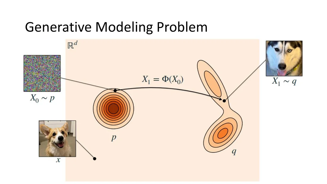
Two kinds of models:

• Direct map $X_1=\Phi (X_0)$ (e.g. GANs): efficient sampling, but not probabilistic and a delicate min-max loss.
• Continuous-time Markov process $(X_t{)}_{0\le t\le 1}$ with $X_{t+h}\leftarrow {\Phi }_{t+h|t}(X_t)$: move the sample step by step. Three kinds of paths: flow (smooth), diffusion (noisy), jump (discontinuous).

Slide 8: flow, diffusion and jump processes.

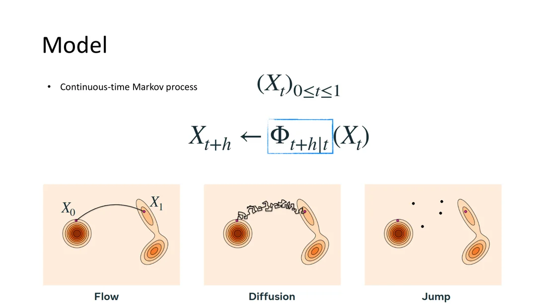
Marginal probability path

Freeze time at $t$: $X_t$ is a random variable with distribution $p_t$, $X_t\sim p_t$. The marginal probability path is the family $\{p_t\}$, a continuous path of distributions from $p_0=p$ to $p_1=q$.

Why focus on flows? They are deterministic (the state at $t+h$ is determined by the state at $t$) and smooth: simple, faster sampling, an exact likelihood estimator, flexible and easier to build. Diffusion and jump processes have a larger design space, but slower sampling and only an ELBO.

Flows and Velocities

Slides 11-17

Flow

$$X_t={\psi }_t(X_0),t\in [0,1]$$

${\psi }_t$: a warping function (a diffeomorphism: a smooth bijection that reshapes space without losing information). $X_0\sim p$: the source. Markov: $X_{t+h}={\psi }_{t+h|t}(X_t)$, the future depends only on the present.

Slide 12: a flow moves samples from a Gaussian through a warping grid.

Flow = velocity. Flows are non-linear (a linear combination of bijections is usually not a bijection), which makes them hard to parameterize. Instead we use the velocity field $u_t(x)$, the local speed and direction:

Flow ↔ velocity

$$\frac{d}{dt}{\psi }_t(x)=u_t({\psi }_t(x))$$

Velocity → flow: solve an ODE (numerical integration). Flow → velocity: differentiate.

• ✓ velocities are linear: averages of velocities are velocities
• ✗ getting samples needs simulation (ODE solving)

Slide 13: the velocity field (blue arrows) deforms the space.

A velocity $u_t$ generates $p_t$ if $X_t={\psi }_t(X_0)\sim p_t$.

Goal and sampling

Train a velocity $u_t^{\theta }$ that generates $p_t$ with $p_0=p$ and $p_1=q$. Sample $X_0\sim p$ and solve

$$\frac{d}{dt}{X}_t=u_t^{\theta }(X_t)$$

from $t=0$ to $t=1$ with any numerical ODE solver (the midpoint method works well).

Simplest Version of Flow Matching

Slides 18-19

Training (simplest version)

1. sample $X_0\sim p$ (noise), $X_1\sim q$ (data), with an arbitrary coupling $(X_0,X_1)\sim {\pi }_{0,1}$ (e.g. independent)
2. sample $t\sim \mathcal{U}[0,1]$
3. interpolate $X_t=(1-t)X_0+t{X}_1$
4. regress the velocity:

$${\mathbb{E}}_{t,X_0,X_1}{\Vert u_t^{\theta }(X_t)-(X_1-X_0)\Vert }^2$$

The code fits in ~10 lines, much less than a diffusion model.

Slide 18: the simplest version of flow matching.

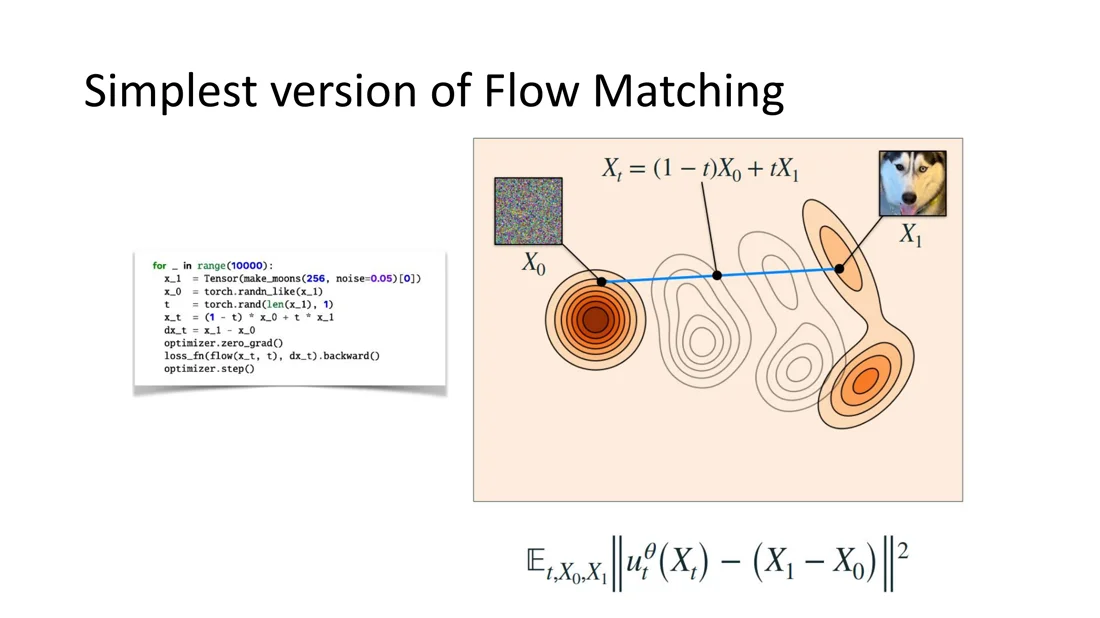
Why does this work, although the pairs $(X_0,X_1)$ are random and even contradictory?

Answer build the flow from conditional flows (each conditioned on one target point), and (2) regress conditional flows, which gives the same gradient as regressing the global flow. The averaged effect of all random pairs is a consistent global flow.

Two ingredients: (1)

Building the Flow from Conditional Flows

Slides 20-23

Generate a single target point $x_1$: the conditional flow moves every point towards $x_1$ (like gravity):

$$X_t={\psi }_t(X_0\mid x_1)=(1-t)X_0+t{x}_1,$$

with conditional probability $p_{t|1}(x\mid x_1)$ and conditional velocity $u_t(x\mid x_1)$.

Average over the data: at $t=0$ all conditional paths start at $p$; at $t=1$ each ends at a delta at its $x_1$. Averaging over all training examples gives a path from $p$ to the (empirical) data distribution $q$. Because velocities are linear, averaging the conditional velocities gives the velocity of the averaged path.

Slides 20-22: a conditional flow towards a single target point.

The marginalization trick (theorem)

The marginal velocity generates the marginal probability path, where

$$u_t(x)=\mathbb{E}\left[u_t(X_t\mid X_1)|X_t=x\right],p_t(x)={\mathbb{E}}_{X_1}{p}_{t|1}(x\mid X_1)$$

Flow Matching Loss

Slide 24

Flow matching (FM) vs. conditional flow matching (CFM)

$${\mathcal{L}}_{FM}(\theta )={\mathbb{E}}_{t,X_t}{\Vert u_t^{\theta }(X_t)-u_t(X_t)\Vert }^2{\mathcal{L}}_{CFM}(\theta )={\mathbb{E}}_{t,X_1,X_t}{\Vert u_t^{\theta }(X_t)-u_t(X_t\mid X_1)\Vert }^2$$

Theorem: the losses are equivalent,

$${\nabla }_{\theta }{\mathcal{L}}_{FM}(\theta )={\nabla }_{\theta }{\mathcal{L}}_{CFM}(\theta )$$

Intuition

We can’t compute the marginal velocity $u_t(x)$ (it averages over the whole data distribution). But we don’t need to: regressing the easy, per-pair conditional velocity gives the same gradient, because the average of the regression targets is exactly the marginal velocity.

How to Choose the Conditional Flow

Slide 25

Optimal transport minimizes the kinetic energy. With Jensen’s inequality:

$${\int }_0^1{\mathbb{E}}_{X_t\sim p_t}\Vert u_t(X_t){\Vert }^{2}dt\le {\mathbb{E}}_{X_0,X_1}{\int }_0^1{\Vert {\dot{\psi }}_t(X_0\mid X_1)\Vert }^{2}dt$$

Linear conditional flow ${\psi }_t(x\mid x_1)=t{x}_1+(1-t)x$:

• minimizes the bound
• reduces the kinetic energy of the initial coupling
• is exact optimal transport for single data points
• is not optimal transport in general (but in high dimensions the paths are straighter)

Flow Matching vs. Diffusion

Slides 26-28

For a Gaussian source distribution, they are different views of the same mechanism. Numerically, diffusion and (linear) flow matching are equivalent up to reparameterization: the noise prediction (diffusion) and the score function (score matching) at a given time $t$ can be converted into a velocity in closed form.

	Diffusion models	Flow matching
Path type	stochastic, noise-added SDE paths	deterministic, ODE-based velocity fields
Training supervision	predict noise / score via a variational objective	direct regression of the velocity field
Sampling cost	thousands of iterative denoising steps	fewer steps (10-100) with ODE solvers
Theoretical robustness	inverse of a 2nd-order PDE; unstable under approximation	1st-order PDE; more stable inversion, small-error behavior
Paths	fixed noise schedules	arbitrary or optimal paths

Summary on flow matching

• Flow matching learns a direct velocity field that transforms noise into data deterministically.
• Diffusion models learn to reverse a stochastic noising process.
• FM can be seen as a generalization of diffusion models, with better sample efficiency, stability and flexibility.
• Under Generator Matching, both are unified: transform distributions along well-defined paths.

Converting a noise prediction into a velocity (linear path)

With $X_t=(1-t)X_0+t{X}_1$ and $X_0=\mathbf{ϵ}$ (noise), the velocity target is $X_1-\mathbf{ϵ}$. If a model predicts the noise $\widehat{\mathbf{ϵ}}$ at $X_t$, then ${\hat{X}}_1=\frac{X_t-(1-t)\widehat{\mathbf{ϵ}}}{t}$ and $\hat{u}={\hat{X}}_1-\widehat{\mathbf{ϵ}}=\frac{X_t-\widehat{\mathbf{ϵ}}}{t}$. So one prediction determines the other: the difference is the parameterization, not the information. (Diffusion’s ${\mathbf{x}}_t=\sqrt{{\bar{\alpha }}_t}{\mathbf{x}}_0+\sqrt{1-{\bar{\alpha }}_t}\mathbf{ϵ}$ is a different, curved schedule of the same kind of interpolation.)

3D Generative Models

Slides 29-30

flowchart TD
  G["3D generative models"] --> O["Optimization-based<br/>SDS: DreamFusion"]
  G --> F["Optimization-free"]
  F --> D["Direct<br/>point cloud diffusion: PC²"]
  F --> L["Latent"]
  L --> S["Structured latents<br/>TRELLIS (SLAT)"]
  L --> U["Unstructured latents<br/>3DShape2VecSet, Hunyuan3D 2.0"]

Score Distillation Sampling

Slides 31-36

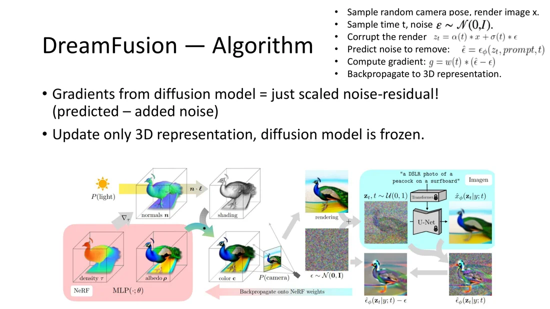
SDS, introduced by DreamFusion: Text-to-3D using 2D Diffusion (Poole et al., 2022): distill 3D information from a 2D diffusion model.

Why use 2D diffusion models for 3D? 2D diffusion models (e.g. Stable Diffusion) are trained on large-scale image-text data; 3D datasets are scarce and costly. Idea: let a pre-trained 2D model guide the optimization of 3D content, without any 3D training data.

Slide 32: DreamFusion results

Slide 32: DreamFusion results

Setup:

• a 3D representation with differentiable rendering (NeRF, Gaussian splatting)
• differentiably render from a random viewpoint
• run the diffusion model on the rendered view, get gradients, backpropagate into the 3D representation

SDS algorithm

1. sample a random camera pose, render an image $\mathbf{x}=g(\theta )$ from the 3D representation $\theta$
2. sample a time $t$ and noise $\mathbf{ϵ}\sim \mathcal{N}(0,\mathbf{I})$
3. corrupt the render: ${\mathbf{z}}_t=\alpha (t)\mathbf{x}+\sigma (t)\mathbf{ϵ}$
4. predict the noise: $\widehat{\mathbf{ϵ}}={\mathbf{ϵ}}_{\varphi }({\mathbf{z}}_t;\text{prompt},t)$
5. compute the gradient: $g=w(t)(\widehat{\mathbf{ϵ}}-\mathbf{ϵ})$
6. backpropagate to the 3D representation:

$${\nabla }_{\theta }{\mathcal{L}}_{SDS}={\mathbb{E}}_{t,\mathbf{ϵ}}\left[w(t)(\widehat{\mathbf{ϵ}}-\mathbf{ϵ})\frac{\partial \mathbf{x}}{\partial \theta }\right]$$

Intuition

The gradient from the diffusion model is just a scaled noise residual (predicted minus added noise): “how would the diffusion model change this render to make it more likely under the prompt?” The diffusion model is frozen; only the 3D representation is updated. The Jacobian of the U-Net is skipped (stop-gradient trick).

Slide 35: the DreamFusion algorithm.

Limitations:

• Janus problem (Janus: the Roman god with two faces): views are optimized independently without global 3D consistency, so the object can get several faces.
• Speed: many diffusion steps until convergence (up to 30 minutes).
• Quality: optimizing from different views averages details.

Slide 36: SDS optimization seen from several views.

(Zero-1-to-3 uses a similar score-distillation loss to reconstruct a neural field: Lecture 10.)

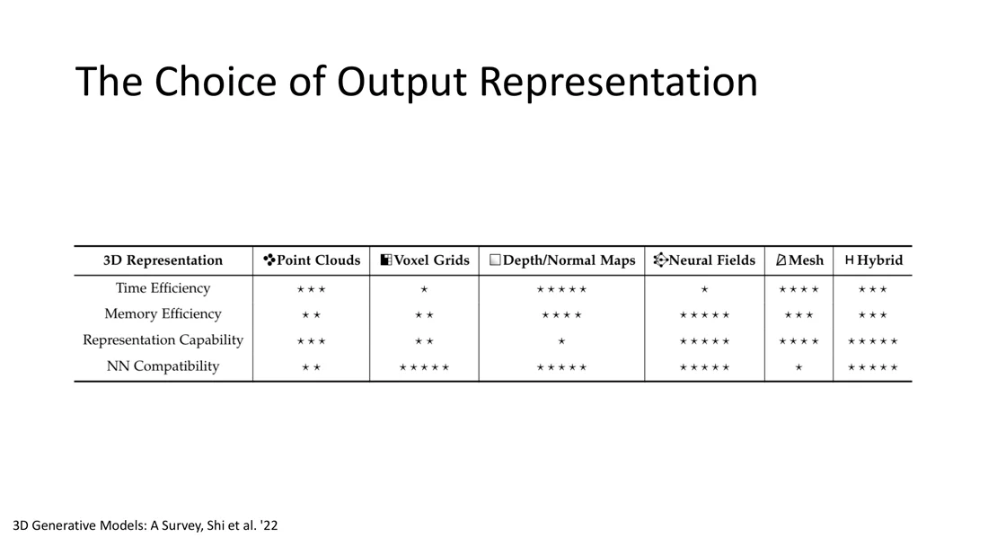
Optimization-Free 3D Generative Models: Design Choices

Slides 37-40

• Input conditions: none, text, images, …
• Output 3D representation: voxels, fields, point clouds, meshes, 3DGS parameters
• Explicit vs. latent diffusion and representation (structured / unstructured latent)
• Generative backbone: GAN, VAE, diffusion, …

For a diffusion model, the output representation matters: diffusion denoises continuous vectors (discrete data like meshes needs workarounds), and it runs hundreds to thousands of steps, so the representation must be efficient and network-friendly.

Slide 39: point clouds, voxel grids, depth/normal maps, neural fields, meshes and hybrids as output representations.

Direct: Image-Conditioned Point Cloud Diffusion (PC²)

Slides 41-45

A direct point cloud diffusion model conditioned on an image. Key idea: enrich the points with projected image features at each diffusion step.

PC²: projection-conditioned diffusion (Melas-Kyriazi et al., CVPR 2023)

• random Gaussian points $p\in {\mathbb{R}}^3$, perspective projection $\pi :{\mathbb{R}}^3\to {\mathbb{R}}^2$
• image encoder $f_{\varphi }:I\in {\mathbb{R}}^{3\times H\times W}\to {\mathbb{R}}^{D\times H^{\prime }\times W^{\prime }}$
• pixel-aligned feature $F_p=f_{\theta }(I)[\pi (p)]$ ($[\cdot ]$: bilinear interpolation)
• diffusion model ${\mathbf{ϵ}}_{\theta }:(F_p,t)\to {\mathbb{R}}^3$ predicts the update for the next step

Slide 43: PC².

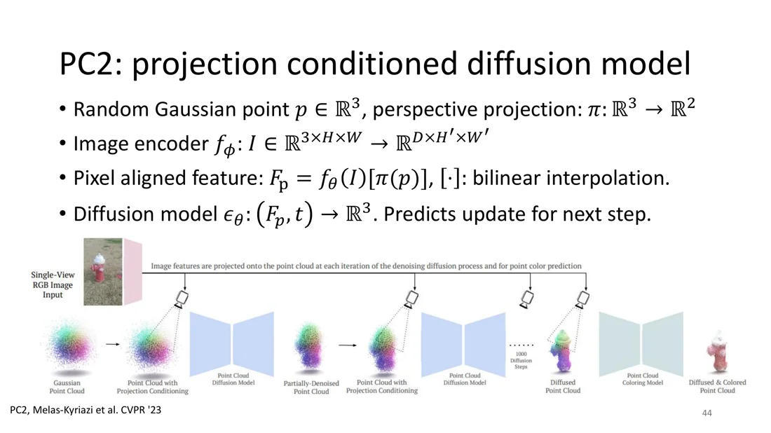
Because it is generative, PC² can produce sharp structures on the back side.

Strengths	Limitations
explicit 3D representation	requires point clouds for training
stable training	cannot perform novel view synthesis
	same limitations as diffusion (slow inference, repeated forward passes)

Latent Diffusion Models for 3D

Slides 46-47

Diffusion models are powerful, but denoising a 3D asset directly may be infeasible:

• high-dimensional data (detailed point clouds, 3DGS parameters)
• discrete (meshes with connectivity) or infinite-dimensional (neural fields, SDFs) representations: what exactly would we denoise?

Instead: compress the data with a pre-trained autoencoder (VAE), perform diffusion in the latent space, and decode back to the original format (like Stable Diffusion). Clever encoders and decoders also solve the discrete/infinite-dimensional problem by mapping to continuous, finite latents.

Structured vs. Unstructured Latents

Slide 48

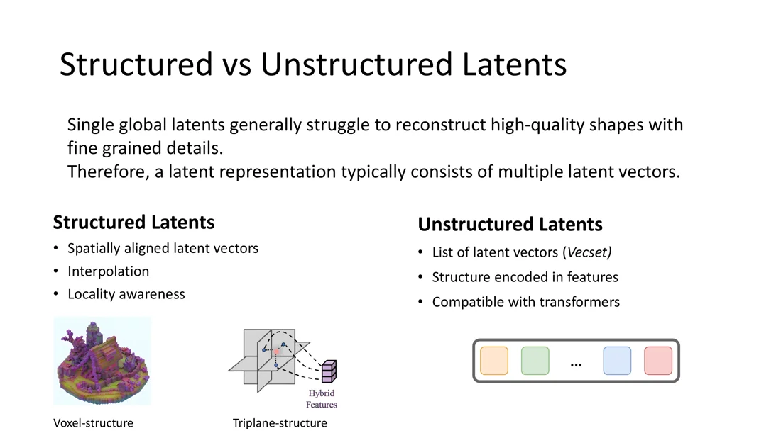
A single global latent generally struggles to reconstruct high-quality shapes with fine details. Therefore a latent representation typically consists of multiple latent vectors.

Structured vs. unstructured latents

	Structured latents	Unstructured latents
What	spatially aligned latent vectors (voxel structure, triplane structure)	a list (set) of latent vectors: a VecSet
Where is the 3D structure?	in the arrangement (the grid)	encoded in the features
Properties	interpolation, locality awareness	compact, compatible with transformers (permutation equivariant)
Processing	3D CNNs / sparse or windowed attention (harder)	standard (cross-)attention
Examples	TRELLIS (SLAT)	3DShape2VecSet, Hunyuan3D 2.0
Best for	fidelity and local editing	simple, compact generation (currently dominant)

Slide 48: structured vs. unstructured latents.

When to use which?

• Structured when you need spatial correspondence: local edits (“change only the roof”), high fidelity, multiple output formats decoded from the same grid, locality-aware processing.
• Unstructured when you want a compact, fixed-size set that a standard transformer can generate; the structure is learned in the features, and a query point reads the shape via cross-attention.
• Summary from the lecture: VecSets = simple, compact, dominant for generation; SLAT = structured, spatial, best for fidelity and editing.

TRELLIS: Voxel-Based Structured 3D Latents

Slides 49-63

TRELLIS (Xiang et al., CVPR 2025, “Structured 3D Latents for Scalable and Versatile 3D Generation”): image-to-3D and text-to-3D, different output formats (3DGS, NeRF, mesh), trained on more than 500,000 assets with models up to 2 billion parameters. State of the art for text- and image-conditioned generation, and it allows flexible editing.

Slide 51: the structured latent (SLAT).

Structured latent (SLAT)

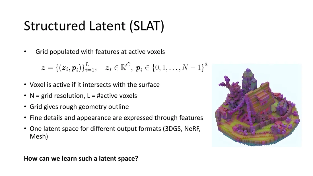
A grid populated with features at active voxels:

$$\mathbf{z}=\{({\mathbf{z}}_i,{\mathbf{p}}_i){\}}_{i=1}^L,{\mathbf{z}}_i\in {\mathbb{R}}^C,{\mathbf{p}}_i\in \{0,1,\dots ,N-1{\}}^3$$

• a voxel is active if it intersects the surface; $N$ = grid resolution, $L$ = number of active voxels
• the grid gives the rough geometry outline
• fine details and appearance are expressed through the features
• one latent space for different output formats (3DGS, NeRF, mesh)

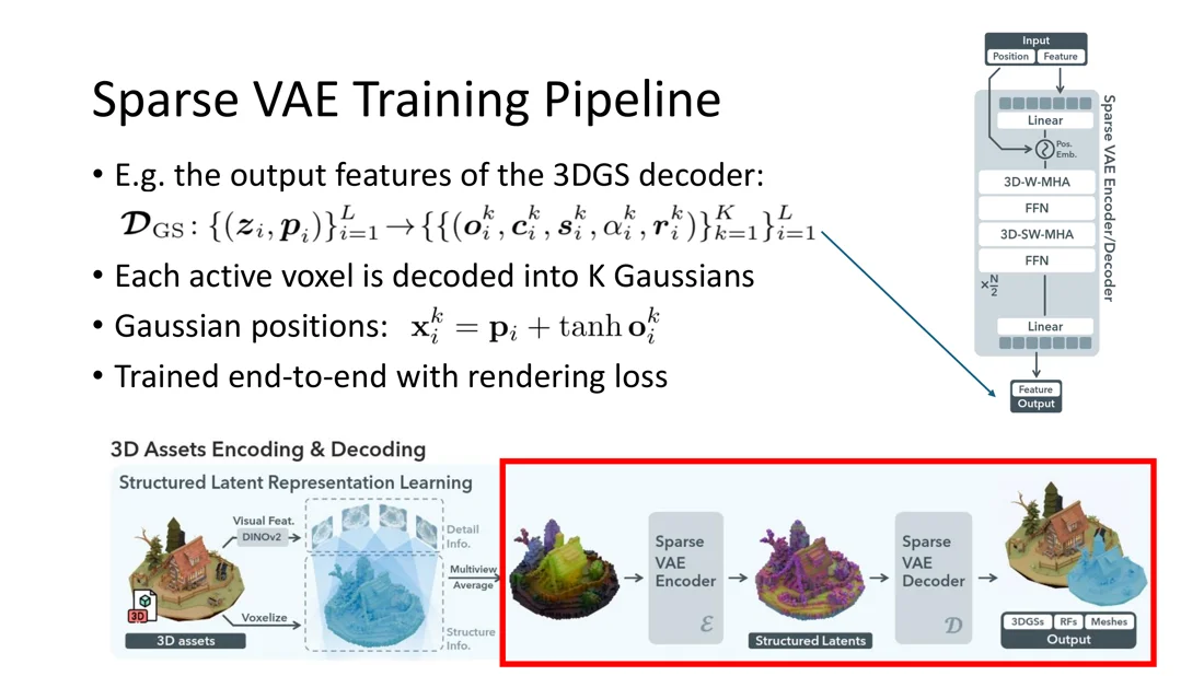
Sparse VAE training pipeline (how the latent space is learned):

1. Voxelize the asset and render it from multiple views.
2. Extract image features (DINOv2) and project them onto the voxels; average over the views → a sparse image-feature volume $\mathbf{f}=\{({\mathbf{f}}_i,{\mathbf{p}}_i){\}}_{i=1}^L$ (not the final latent yet!).
3. A sparse VAE encoder (transformer with shifted-window attention for locality and efficiency) turns it into the SLAT $\mathbf{z}$.
4. Specific decoders for different output formats. E.g. the 3DGS decoder decodes each active voxel into $K$ Gaussians,

$${\mathcal{D}}_{GS}:\{({\mathbf{z}}_i,{\mathbf{p}}_i){\}}_{i=1}^L\to \{\{({\mathbf{o}}_i^k,{\mathbf{c}}_i^k,{\mathbf{s}}_i^k,{\alpha }_i^k,{\mathbf{r}}_i^k){\}}_{k=1}^K{\}}_{i=1}^L,{\mathbf{x}}_i^k={\mathbf{p}}_i+\tanh {\mathbf{o}}_i^k$$

($\tanh \in (-1,1)$ keeps each Gaussian close to its voxel), trained end-to-end with a rendering loss.

In practice the encoder is trained together with the 3DGS decoder; the NeRF and mesh decoders are trained afterwards with the encoder frozen.

Slide 54: the sparse VAE pipeline.

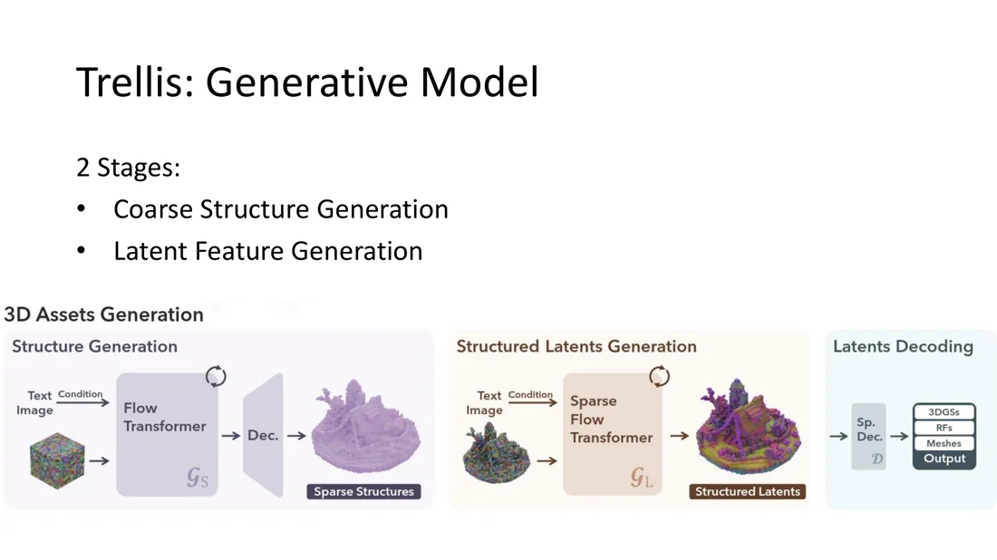
Generative model: learn to generate the structured latent, in 2 stages.

1. Coarse structure generation: generating the occupancy grid $\mathbf{O}\in \{0,1{\}}^{N\times N\times N}$ directly is expensive. Instead, a 3D convolutional VAE compresses it into a feature volume $\mathbf{S}\in {\mathbb{R}}^{D\times D\times D\times C_S}$; a flow transformer ${\mathcal{G}}_S$ generates $\mathbf{S}$ (conditions injected via cross-attention), which is decoded into the active voxels. The continuous feature volume also suits diffusion/flow models better than binary occupancy.
2. Latent feature generation: a second (sparse) flow transformer ${\mathcal{G}}_L$ generates the features ${\mathbf{z}}_i$ at the active voxels.

Then the decoders turn the SLAT into 3DGS, NeRF or a mesh.

Slide 58: the two-stage generative model.

Slide 61: TRELLIS results

Slide 62: text-to-3D with TRELLIS

TRELLIS key takeaways

• trained on 0.5 M assets, 2 B parameter models
• structured latent representation with spatial awareness
• a coarse structure equipped with features that encode fine details and appearance
• the spatial representation allows local editing
• multiple output formats via distinct decoders
• a latent model that generates high-quality assets from text or images

Unstructured Latents: 3DShape2VecSet

Slides 64-73

3DShape2VecSet (Zhang et al., SIGGRAPH 2023). Key idea: encode a 3D object as a set of latent vectors, then predict a signed distance (or occupancy) field. How do we predict a set? With a cross-attention transformer, which is permutation equivariant.

Slide 68: shape encoding, KL regularization and shape decoding.

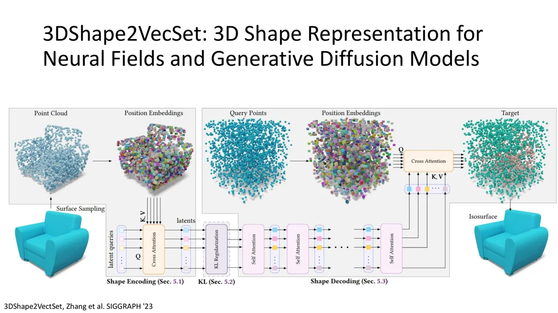
Encoder: sample points on the shape surface, enrich them with a positional embedding (${\mathbb{R}}^3\to {\mathbb{R}}^C$), and cross-attend from a set of latent queries:

1. learnable latent queries $\mathbf{L}\in {\mathbb{R}}^{C\times M}$: ${\text{Enc}}_{learnable}(\mathbf{X})=\text{CrossAttn}(\mathbf{L},\text{PosEmb}(\mathbf{X}))\in {\mathbb{R}}^{C\times M}$
2. subsampled latent queries via farthest point sampling (as in PointNet++): ${\mathbf{X}}_0=\text{FPS}(\mathbf{X})\in {\mathbb{R}}^{3\times M}$, ${\text{Enc}}_{points}(\mathbf{X})=\text{CrossAttn}(\text{PosEmb}({\mathbf{X}}_0),\text{PosEmb}(\mathbf{X}))$

KL regularizer: a linear projection produces a mean and a variance per latent (like a VAE), so a diffusion model can be trained on smaller latents:

$${\mathcal{L}}_{reg}(\{{\mathbf{f}}_i{\}}_{i=1}^M)=\frac{1}{M\cdot C_0}\sum _{i=1}^M\sum _{j=1}^{C_0}\frac{1}{2}\left({\mu }_{i,j}^2+{\sigma }_{i,j}^2-\log {\sigma }_{i,j}^2\right)$$

It makes the latent space Gaussian-like, so similar shapes get similar codes and sampling works.

Decoder: a series of self-attention blocks gives the VecSet $\{{\mathbf{f}}_i{\}}_{i=1}^M$. To evaluate the occupancy at a query point $\mathbf{x}\in {\mathbb{R}}^3$, interpolate the latents via cross-attention, then one fully connected layer:

$$\hat{\mathcal{F}}(\mathbf{x})=\sum _{i=1}^{M}v({\mathbf{f}}_i)\cdot \text{softmax}(\mathbf{q}(\mathbf{x}{)}^T\mathbf{k}({\mathbf{f}}_i)/\sqrt{d}),\mathcal{O}(\mathbf{x})=\text{FC}(\hat{\mathcal{F}}(\mathbf{x}))$$

The surface is extracted with marching cubes.

Trained on ShapeNet (lamps, chairs, cars, …): reconstruction from point clouds and generation conditioned on categories, text, partial observations or images. Its full potential shows in Hunyuan3D.

Hunyuan3D 2.0

Slides 74-79

Hunyuan3D 2.0 (Tencent Hunyuan 3D team, 2025), a state-of-the-art image-to-3D model with two parts:

1. Shape generation (Hunyuan3D-DiT): a high-fidelity, textureless mesh from an input image. A latent diffusion model.
2. Texture synthesis (Hunyuan3D-Paint): the matching texture.

Slide 74: Hunyuan3D 2.0.

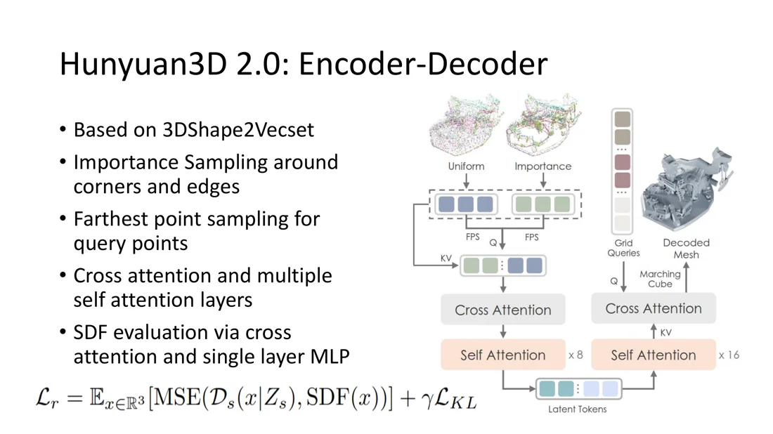
Encoder-decoder (ShapeVAE): based on 3DShape2VecSet, with importance sampling around corners and edges, farthest point sampling for query points, cross-attention and multiple self-attention layers, and SDF evaluation via cross-attention and a one-layer MLP:

$${\mathcal{L}}_r={\mathbb{E}}_{x\in {\mathbb{R}}^3}\left[\text{MSE}\right({\mathcal{D}}_s(x\mid Z_s),\text{SDF}(x)\left)\right]+\gamma {\mathcal{L}}_{KL}$$

Hunyuan3D-DiT: a flow-based diffusion model (a denoising transformer on the latent tokens), conditioned on the image:

$$\mathcal{L}={\mathbb{E}}_{t,x_0,x_1}[\Vert u_{\theta }(x_t,c,t)-u_t{\Vert }_2^2],u_t=\frac{d{x}_t}{dt},t\sim \mathcal{U}(0,1)$$

($c$: the model condition). This is the flow matching loss from the first part of the lecture.

Hunyuan3D-Paint: a multi-view diffusion network generates the textures, conditioned on renders of normals and positions of the generated mesh and on the input image (with image de-lighting, a reference branch and multi-task attention).

Slide 76: Hunyuan3D 2.0 encoder-decoder.

Conclusion

Slide 81

• Flow matching
• 3D generation and reconstruction:
  • SDS-based methods: distilling 3D from 2D diffusion
  • point cloud diffusion
  • TRELLIS: mapping 2D features to structured 3D voxels
  • 3DShape2VecSet and Hunyuan: compressing shapes into an unstructured latent vector set
• VecSets = simple, compact, dominant for generation; SLAT = structured, spatial, best for fidelity and editing.

Method	Family	Representation	Needs 3D training data?
DreamFusion (SDS)	optimization-based	NeRF / 3DGS, optimized per prompt	no (2D diffusion)
PC²	direct diffusion	point cloud	yes
TRELLIS	latent (structured)	sparse voxel features → 3DGS / NeRF / mesh	yes
3DShape2VecSet, Hunyuan3D 2.0	latent (unstructured)	vector set → SDF → mesh	yes

Transfer: Depth and the Back of a Scene with Diffusion

The exam hint asks to “put together pieces, with diffusion, to reconstruct depth and the back part of a scene, based on the algorithms you’ve seen”. One possible combination from the course:

flowchart LR
  I["single image"] --> D["depth: monocular depth<br/>(Depth Anything) or<br/>DUSt3R with the image twice"]
  I --> MV["back views: multi-view diffusion<br/>(Zero-1-to-3), conditioned on (R, T)"]
  D --> P["visible geometry<br/>(point map)"]
  MV --> R["3D reconstruction from all views<br/>(DUSt3R / 3DGS), keep consistent<br/>e.g. Gen-3Diffusion style"]
  P --> R
  R --> O["full 3D scene incl. back"]

• The visible part comes from depth (Lecture 4) or point maps (Lecture 9).
• The hidden back is ill-posed, so it must be generated: multi-view diffusion or a 3D generative model (TRELLIS / Hunyuan3D) conditioned on the image.
• Consistency between generated views needs an explicit 3D representation (Gen-3Diffusion) or SDS with a single 3D model.

Self-Test

What is the idea of flow matching in one sentence?

Answer $\frac{d}{dt}{X}_t=u_t^{\theta }(X_t)$).

Train a network by regressing a velocity field that transports noise to data; generate by following that velocity (solving the ODE

Why parameterize velocities instead of flows?

Answer

Flows are bijections and non-linear; averaging two flows usually gives no flow. Velocities are linear, so averages of velocities are valid velocities. The price: sampling requires solving an ODE.

Write down the simplest flow matching training step.

Answer $X_0\sim p$, $X_1\sim q$, $t\sim \mathcal{U}[0,1]$; $X_t=(1-t)X_0+t{X}_1$; minimize $\Vert u_t^{\theta }(X_t)-(X_1-X_0){\Vert }^2$.

Sample

Why does training with random pairs work?

Answer ${\nabla }_{\theta }{\mathcal{L}}_{FM}={\nabla }_{\theta }{\mathcal{L}}_{CFM}$, so regressing per-pair conditional velocities gives the right gradient.

The marginal velocity is the conditional expectation of the conditional velocities and generates the marginal probability path (marginalization trick), and

Contrast flow matching and diffusion.

Answer

Diffusion: stochastic SDE paths, predicts noise/score via a variational objective, thousands of steps, inverts a 2nd-order PDE, fixed noise schedule. Flow matching: deterministic ODE, regresses the velocity directly, 10-100 steps, 1st-order PDE (more stable), arbitrary paths. For a Gaussian source they are equivalent up to reparameterization.

How does score distillation sampling work, and what are its limitations?

Answer $w(t)(\widehat{\mathbf{ϵ}}-\mathbf{ϵ})\frac{\partial \mathbf{x}}{\partial \theta }$ into the 3D representation. Limitations: Janus problem (multiple faces), slow (up to 30 min), averaged details.

Render a random view of a 3D representation, add noise, let a frozen 2D diffusion model predict the noise, and backpropagate

What is the difference between structured and unstructured latents? When would you use which?

Answer

Structured: latents aligned in space (voxels, triplanes), with locality and interpolation; good for fidelity, local editing and multiple output formats (TRELLIS). Unstructured: a set of latent vectors whose features encode the structure; compact and transformer-friendly; dominant for generation (3DShape2VecSet, Hunyuan3D).

What is SLAT, and how does TRELLIS learn and generate it?

Answer $\mathbf{z}=\{({\mathbf{z}}_i,{\mathbf{p}}_i){\}}_{i=1}^L$: features at active (surface) voxels. Learned with a sparse VAE: voxelize, project and average DINOv2 features from rendered views, encode with shifted-window attention, decode with format-specific decoders (e.g. $K$ Gaussians per voxel). Generated in two stages with flow transformers: coarse structure (compressed occupancy volume), then the latent features.

How does 3DShape2VecSet encode and decode a shape?

Answer

Encode: positional embeddings of surface points, cross-attention from learnable or FPS-sampled latent queries, KL-regularized projection. Decode: self-attention blocks give the VecSet; a query point cross-attends to it and an FC layer gives occupancy/SDF; marching cubes extracts the surface.

What are the two parts of Hunyuan3D 2.0?

Answer

Shape generation: a VecSet-based ShapeVAE plus a flow-based diffusion transformer (Hunyuan3D-DiT) conditioned on the image. Texture synthesis: multi-view diffusion (Hunyuan3D-Paint) conditioned on normal and position renders and the input image.

Related

• Previous: Lecture 10: Diffusion Models · Course: Overview
• Concepts: Flow Matching, Diffusion Model, Neural Field, Gaussian Splatting, Signed Distance Function, Attention, PointNet
• Structured feature grids and triplanes: Lecture 6.1. Farthest point sampling: Lecture 6.2.