Lecture 7: Neural Radiance Fields (NeRF)

TL;DR

1. NeRF solves novel view synthesis: from a sparse set of images with known camera poses, render new views of the same scene.
2. An MLP $F_{\theta }:(x,y,z,\theta ,\varphi )\mapsto (r,g,b,\sigma )$ stores color and volume density for every 3D point and viewing direction.
3. The scene is a cloud of tiny colored particles. $\sigma (t)dt$ is the probability that a ray stops at $t$; the transmittance $T(t)$ is the probability of getting there. The pixel color is the expected color under the PDF $T(t)\sigma (t)$.
4. Discretized, this is alpha compositing: $\hat{C}={\sum }_i{T}_i{\alpha }_i{\mathbf{c}}_i$ with ${\alpha }_i=1-e^{-{\sigma }_i{\delta }_i}$ and $T_i={\prod }_{j<i}(1-{\alpha }_j)$. It is differentiable, so NeRF is trained with a photometric loss on 2D images.
5. Without positional encoding (Fourier features) the results are blurry.
6. Limitations: static scenes only, no editing, no generalization, slow, inaccurate surfaces. Variants fix one each: D-NeRF (dynamic), NeRF-W (internet photos), Control-NeRF (editing), Instant NGP (speed), UniSurf (surfaces).

Exam relevance

Highest priority. Exam task 4: both rendering formulas (NeRF and 3D Gaussian Splatting) were given; explain every symbol ($\sigma$, $\alpha$, $T$, $\mathbf{c}$, …) and compare NeRF and 3DGS (similarities and differences). See NeRF vs. 3D Gaussian Splatting and Volume Rendering in NeRF.

Slide 2: scenes reconstructed with NeRF.

Overview: NeRF (2020), the foundational breakthrough · D-NeRF (2021), dynamic NeRF · HyperNeRF (2021), topological dynamics · NeRF-W (2021), unconstrained capture · Control-NeRF (2023), scene manipulation · Instant NGP (2022), training speed. (HyperNeRF appears in the overview, but its slides are hidden and not in the PDF.)

NeRF: The Foundational Breakthrough

Novel View Synthesis

Slides 4-6

Problem: view interpolation / novel view synthesis. Input: sparsely sampled images of a scene. Learn a scene representation. Output: novel views of the scene. (NeRF, Mildenhall et al., ECCV 2020.)

Instead of learning the scene geometry directly, NeRF learns a radiance field: a neural network $F_{\theta }$ that takes a 3D point and a camera viewing direction and predicts a color and a density at that point. Volume rendering then turns this into an image.

Radiance field

$$F_{\theta }:(x,y,z,\theta ,\varphi )⟼(r,g,b,\sigma )$$

Input: spatial location $(x,y,z)$ + viewing direction $(\theta ,\varphi )$ (5D). Output: color $(r,g,b)$ + density $\sigma$.

Slide 5: learning a radiance field representation of the scene.

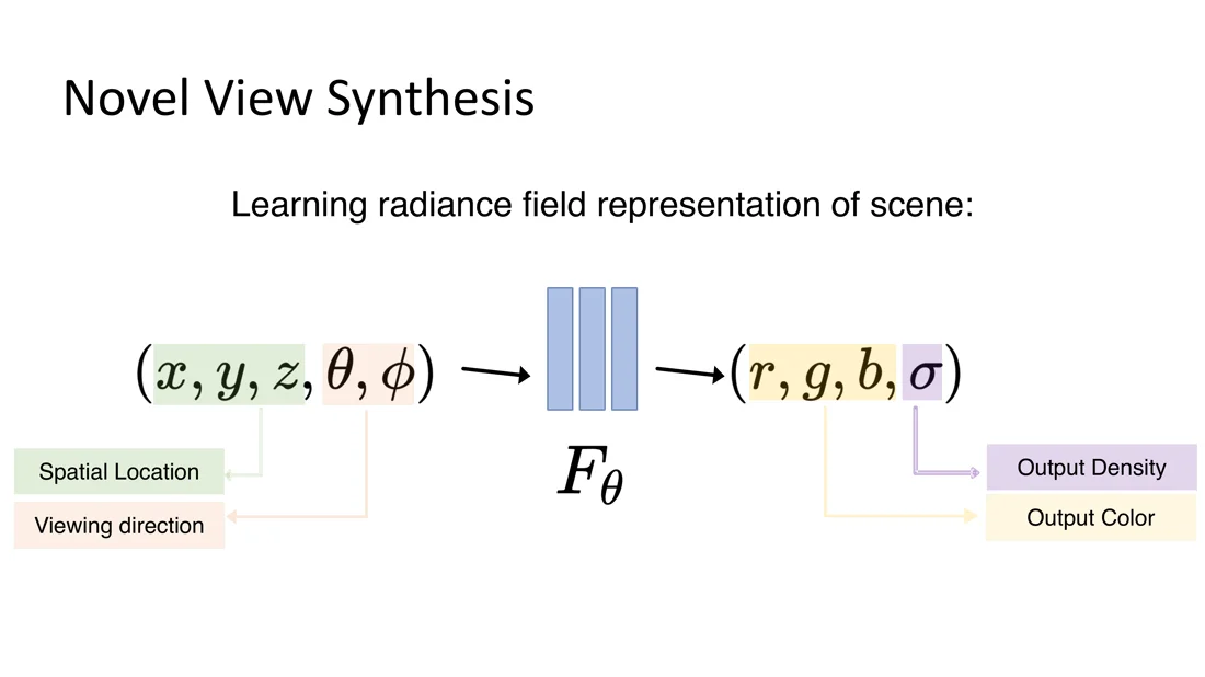
Volume rendering (continuous)

Given color and density, the color of every camera ray is

$$C(\mathbf{r})={\int }_{t_n}^{t_f}T(t)\sigma (\mathbf{r}(t))\mathbf{c}(\mathbf{r}(t),\mathbf{d})dt,T(t)=\exp \left(-{\int }_{t_n}^t\sigma (\mathbf{r}(s))ds\right),\mathbf{r}(t)=\mathbf{o}+t\mathbf{d}$$

Symbol	Meaning
$C(\mathbf{r})$	color of the camera ray (the rendered pixel)
$\mathbf{r}(t)=\mathbf{o}+t\mathbf{d}$	camera ray: $\mathbf{o}$ camera center, $\mathbf{d}$ direction
$t_n,t_f$	near and far bounds
$\mathbf{c}(\mathbf{r}(t),\mathbf{d})$	color $(r,g,b)$ at $\mathbf{r}(t)$ (view-dependent, from the MLP)
$\sigma (\mathbf{r}(t))$	volume density: probability of a ray terminating at an infinitesimal particle at $\mathbf{r}(t)$ (from the MLP)
$T(t)$	accumulated transmittance along the ray: probability that the ray travels from $t_n$ to $t$ without hitting any particle

Intuition

A high density gives a high color contribution, but only if the transmittance is also high. Once the ray has hit a high-density region (inside a surface), $T$ becomes small, and everything behind it contributes nothing. The equation contains both: how dense a point is, and how likely the ray made it that far.

Trap

The upper limit of the inner integral of $T(t)$ is $t$, not $t_f$ (the speaker notes write $t_f$). Otherwise $T$ would be constant along the ray. $T$ is not an output of the MLP; it is accumulated from $\sigma$.

Radiance, Volumetric Radiance and Density

Slides 7-10

Radiance

Radiance is (differential) energy per unit area, solid angle and wavelength: the density of photons at a point, traveling in a given direction, at a given wavelength (= color):

$$L(\mathbf{x},\mathbf{\omega },\lambda ):{\mathbb{R}}^3\times {\mathbb{S}}^2\times \mathbb{R}\mapsto {\mathbb{R}}^{+}$$

• Radiance along an unblocked ray is constant (energy conservation).
• The light field is the radiance for every possible ray.

Volumetric radiance

The scene is a cloud of tiny colored particles. Their color changes according to the viewpoint. If a ray traveling through the scene hits a particle at $t$, we return its radiance/color $\mathbf{c}(t)$.

Volumetric density

The probability that the ray stops in a small interval around $t$ is $\sigma (t)dt$. $\sigma$ is also called volume(tric) density.

Slide 8: volumetric radiance

Slide 9: volumetric density

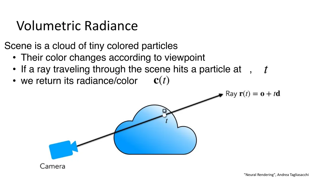
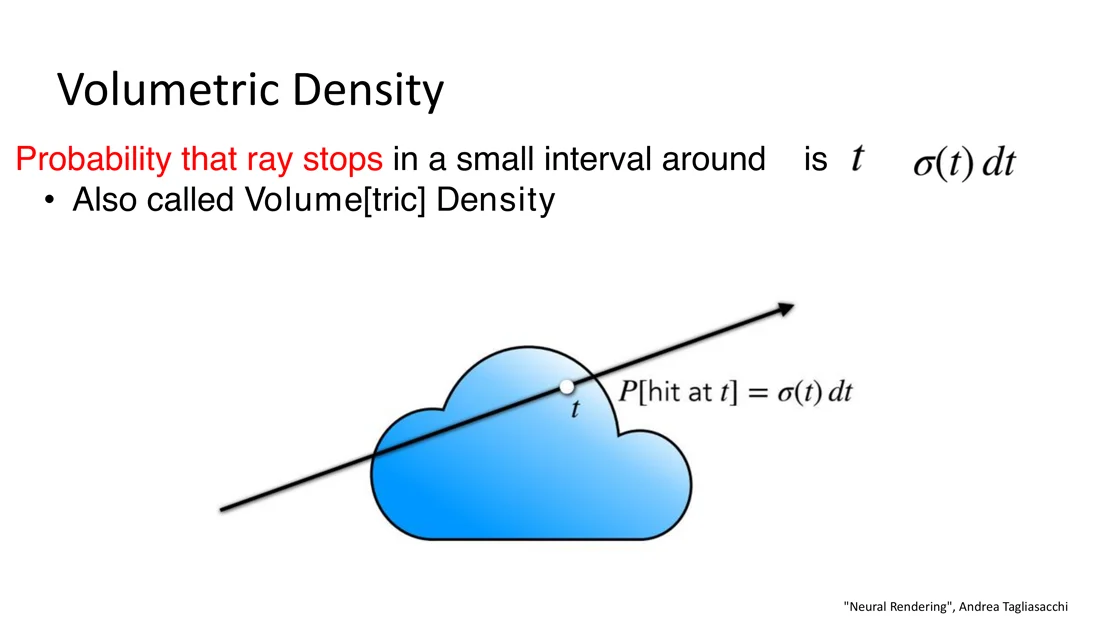
Scene representation: a field (neural? maybe)

$$\Phi :{\mathbb{R}}^3\to {\mathbb{R}}^3\times {\mathbb{R}}^{+},\Phi (\mathbf{x})=(\sigma ,\mathbf{c})$$

While evaluating the field along a ray, we retrieve the color $\mathbf{c}(t)$ only if $\mathbf{r}(t)$ is visible. The transmittance $T(t)$ is the probability that no particle is hit in $[0,t)$. (See Neural Field.)

Trap

$\sigma$ is a density ($\ge 0$, unit 1/length), not a probability; $\sigma dt$ is the probability. $\sigma$ can be larger than 1.

Transmittance and Expected Ray Termination

Slides 11-14

Relating $\sigma$ and $T$: hit probabilities are statistically independent along the ray ($P[A,B]=P[A]P[B]$):

$$P[\text{no hit before }t+dt]=P[\text{no hit before }t]\times P[\text{no hit at }t]⟹T(t+dt)=T(t)(1-\sigma (t)dt)$$

Derivation of the transmittance (Slide 12)

$$\frac{T(t+dt)-T(t)}{dt}=-T(t)\sigma (t)\Rightarrow T^{\prime }(t)=-T(t)\sigma (t)\Rightarrow \frac{T^{\prime }(t)}{T(t)}=-\sigma (t)$$ $${\int }_a^b\frac{T^{\prime }(t)}{T(t)}dt=-{\int }_a^b\sigma (t)dt\Rightarrow \log T(t){|}_a^b=-{\int }_a^b\sigma (t)dt\Rightarrow T(a\to b):=\frac{T(b)}{T(a)}=\exp \left(-{\int }_a^b\sigma (t)dt\right)$$

Transmittance

$$T(0\to t):=T(t)=\exp \left(-{\int }_0^t\sigma (u)du\right)$$

No hits before $t$ is the exponential of the integral over the density up to $t$.

Intuition

Survival multiplies, density adds. Because the hits are independent, the survival probabilities of consecutive pieces multiply; in the limit, the product becomes the exponential of an integral.

Expected ray termination (Slide 13):

• $1-T(t)$ is a cumulative distribution function (CDF): the probability that the ray hits something before reaching $t$. It is non-decreasing, $T$ is (right) continuous, ${\lim }_{t\to -\infty }(1-T(t))=0$, ${\lim }_{t\to \infty }(1-T(t))=1$.
• $\tau (t)=T(t)\sigma (t)$ is a probability density function (PDF): the probability that a ray stops at $t$.

Volume rendering as an expectation (Slide 14)

$$C={\int }_0^{\infty }T(t)\sigma (t)\mathbf{c}(t)dt,T(t)=\exp \left(-{\int }_0^t\sigma (u)du\right)$$

The expected color along a ray is a convex combination of colors, weighted by the probability that the ray stops there.

How do we solve this? Discretize the nested integral.

Discretization: NeRF as Alpha Blending

Slides 15-19

Approximating the integral: split the ray into $N$ segments with endpoints $\{t_1,t_2,\dots ,t_{N+1}\}$. The segment length is ${\delta }_i=t_{i+1}-t_i$.

Warning

The segments are not necessarily uniform. A piecewise constant density does not give a piecewise constant transmittance.

Approximating the nested integral: assume the volume density and color are constant within each interval (a Riemann sum):

$$C={\int }_0^{\infty }T(t)\sigma (t)\mathbf{c}(t)dt\approx \sum _{i=1}^N{\int }_{t_i}^{t_{i+1}}T(t){\sigma }_i{\mathbf{c}}_{i}dt$$

Forward model of NeRF step by step (Slide 17)

$$\begin{array}{rlrl}& \sum _{n=1}^N{\int }_{t_n}^{t_{n+1}}T(t){\sigma }_n{\mathbf{c}}_{n}dt& & \\ & =\sum _{n=1}^N{\int }_{t_n}^{t_{n+1}}T(0\to t_n)T(t_n\to t){\sigma }_n{\mathbf{c}}_{n}dt& & \text{(independent process)}\\ & =\sum _{n=1}^{N}T(0\to t_n){\int }_{t_n}^{t_{n+1}}T(t_n\to t){\sigma }_n{\mathbf{c}}_{n}dt& & \text{(constant)}\\ & =\sum _{n=1}^N{T}_n(1-\exp (-{\sigma }_n{\delta }_n)){\mathbf{c}}_n,T_n=\exp \left(\sum _{k=1}^{n-1}-{\sigma }_k{\delta }_k\right)& & \text{(tedious)}\end{array}$$

Split $T(t)$ into “reach $t_n$” and “from $t_n$ to $t$” (independence). $T(0\to t_n)=T_n$ is constant inside the segment. With constant ${\sigma }_n$, ${\int }_{t_n}^{t_{n+1}}{\sigma }_n{e}^{-{\sigma }_n(t-t_n)}dt=1-e^{-{\sigma }_n{\delta }_n}$. (The speaker notes say “iid”, but only independence is needed.)

NeRF as alpha blending (Slide 18)

$$C=\sum _{n=1}^N{T}_n{\alpha }_n{\mathbf{c}}_n,{\alpha }_n=1-\exp (-{\sigma }_n{\delta }_n)\text{(segment opacity)},T_n=\prod _{k=1}^{n-1}(1-{\alpha }_k)\text{(segment occlusion)}$$

Slide 18: NeRF as alpha blending.

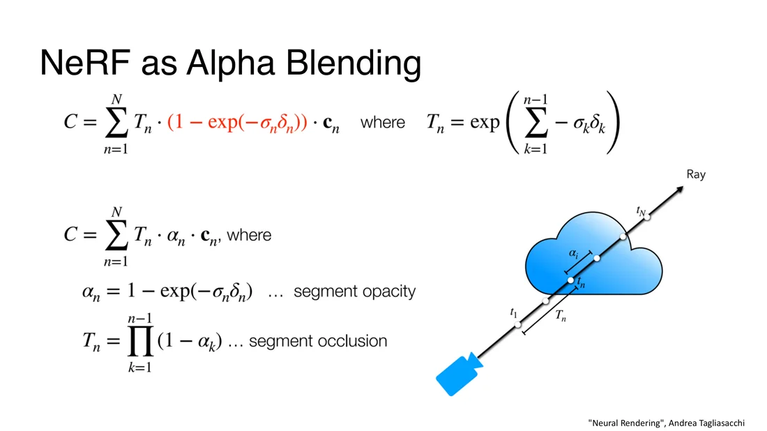
Volume Rendering in NeRF

Slide 19

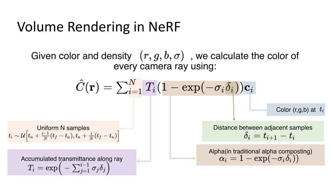
This is the formula to know by heart (and to explain symbol by symbol):

Discrete volume rendering in NeRF

$$\hat{C}(\mathbf{r})=\sum _{i=1}^N{T}_i(1-\exp (-{\sigma }_i{\delta }_i)){\mathbf{c}}_i$$ $$T_i=\exp \left(-\sum _{j=1}^{i-1}{\sigma }_j{\delta }_j\right),{\alpha }_i=1-\exp (-{\sigma }_i{\delta }_i),{\delta }_i=t_{i+1}-t_i,t_i\sim \mathcal{U}\left[t_n+\frac{i-1}{N}(t_f-t_n),t_n+\frac{i}{N}(t_f-t_n)\right]$$

Symbol	Meaning
$\hat{C}(\mathbf{r})$	estimated color of ray $\mathbf{r}$ (the pixel)
$N$	number of samples along the ray
$t_i$	sample positions: uniformly random within $N$ evenly spaced bins between $t_n$ and $t_f$
${\delta }_i$	distance between adjacent samples (not uniform)
${\sigma }_i$	volume density at sample $i$ (MLP output)
${\mathbf{c}}_i$	color $(r,g,b)$ at $t_i$ (MLP output, view-dependent)
${\alpha }_i$	alpha (as in traditional alpha compositing): probability that the ray stops within segment $i$; computed from ${\sigma }_i$ and ${\delta }_i$, in $[0,1)$
$T_i$	accumulated transmittance: probability that the ray reaches sample $i$; sum/product only up to $i-1$

Slide 19: volume rendering in NeRF, every term labeled.

Common mistakes

• $T_i$ sums only up to $i-1$, not $i$.
• In NeRF, ${\alpha }_i$ is not a network output; it is computed from ${\sigma }_i$ and ${\delta }_i$ (in 3DGS, the opacity is learned).
• The samples are not equally spaced; only the bins are.
• Why not simply $T_i{\sigma }_i{\delta }_i$? Because ${\sigma }_i{\delta }_i$ can exceed 1, while ${\alpha }_i$ is always a valid probability.

Training Neural Radiance Fields

Slides 20-22

Training loop

1. March camera rays through the scene to generate a sampled set of 3D points.
2. Use those points and their 2D viewing directions as input to the network to produce colors and densities.
3. Use classical volume rendering to accumulate them into a 2D image.
4. Minimize the error between the rendered color and the ground-truth color:

$$\mathcal{L}=\sum _{\mathbf{r}}{\Vert \hat{C}(\mathbf{r})-C(\mathbf{r})\Vert }_2^2$$

Slide 20: training neural radiance fields.

Slide 21: a ray is sampled, every sample is fed to F_θ, and the colors and densities are composited into a pixel (played 1.5x).

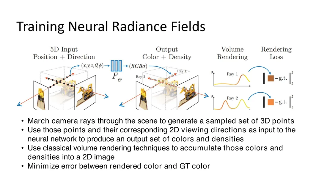
The rendering function is differentiable, so the scene representation is optimized by minimizing the residual between synthesized and observed images.

flowchart LR
  P["camera pose"] --> R["rays r = o + t d"] --> S["samples t_i"] --> E["positional encoding<br/>γ(x), γ(d)"] --> M["MLP F_θ"] --> O["(c_i, σ_i)"] --> V["Σ T_i α_i c_i"] --> C["pixel color Ĉ(r)"]
  C -- "training only" --> L["loss vs. GT pixel<br/>backprop, update θ"]

	Training time	Inference time
Input	photos with known camera poses (e.g. from COLMAP)	a new camera pose
What happens	render, photometric loss, backpropagation	only render
What is learned	the MLP weights $\theta$ (one network per scene)	nothing

View-dependent illumination: the viewing direction $(\theta ,\varphi )$ lets the color change with the view, e.g. specular reflections on a table or screen.

Slide 22: effect of θ and φ on the output field.

Positional Encoding

Slides 23-28

Plain NeRF gives blurry results. Why? Coordinate-based networks fail to learn high-frequency details, for all kinds of data: RGB images, 3D shapes, density, radiance fields.

Slide 24: why blurry results?

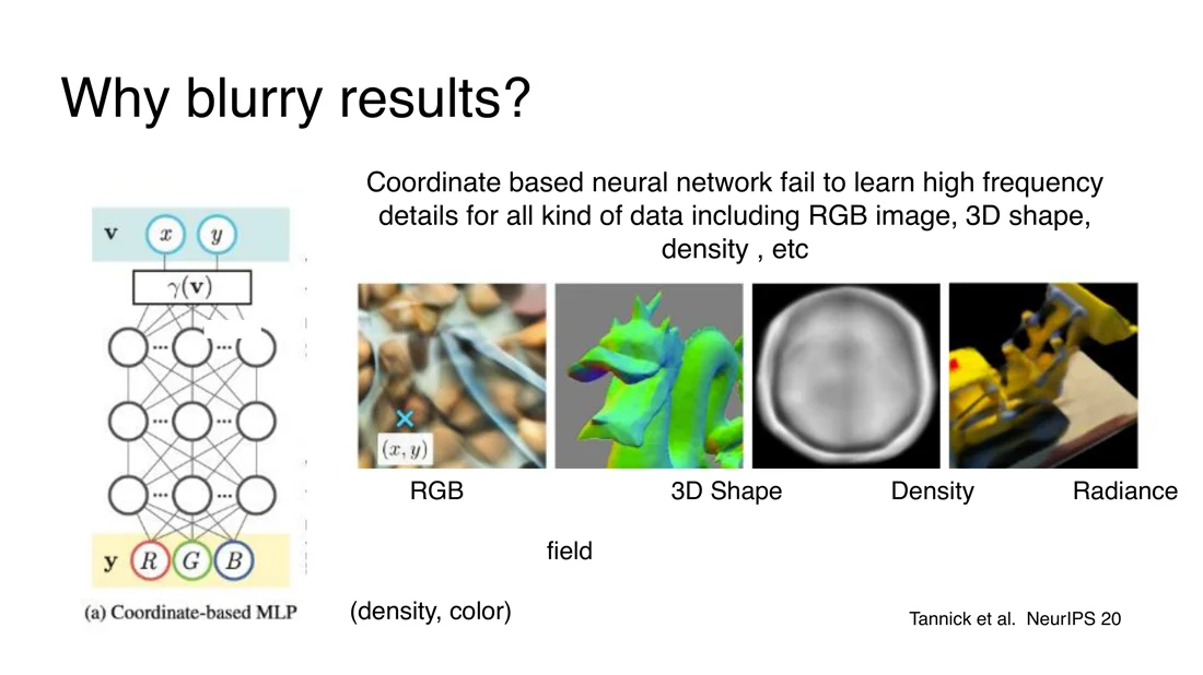
Solution (Tancik et al., NeurIPS 2020, “Fourier Features”):

• In the naive setting, the bandwidth of the Neural Tangent Kernel limits the spectrum of the learned function.
• A Fourier feature mapping turns the neural kernel into a stationary kernel in the low-dimensional input domain and increases the spectrum.

Positional encoding

$$\gamma (p)=(\sin (2^0\pi p),\cos (2^0\pi p),\dots ,\sin (2^{L-1}\pi p),\cos (2^{L-1}\pi p))$$

applied to each coordinate input $p$ (pixel location for images, 3D point for NeRF).

Slide 26: with Fourier features

Slide 27: positional encoding in NeRF

Slide 28: without positional encoding

Slide 28: with positional encoding (Mueller et al., SIGGRAPH 2022)

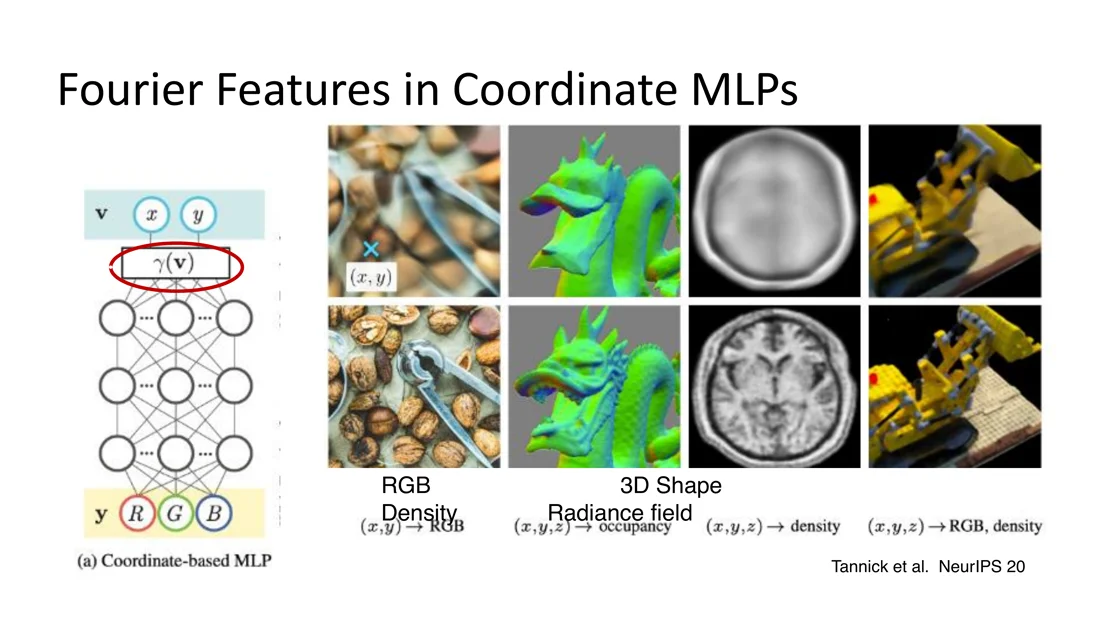
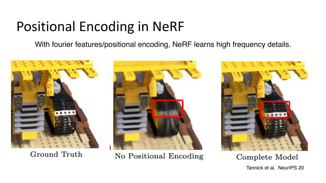
With positional encoding, the network converges much faster and learns the exact appearance of the scene.

Geometry and Results

Slides 29-30

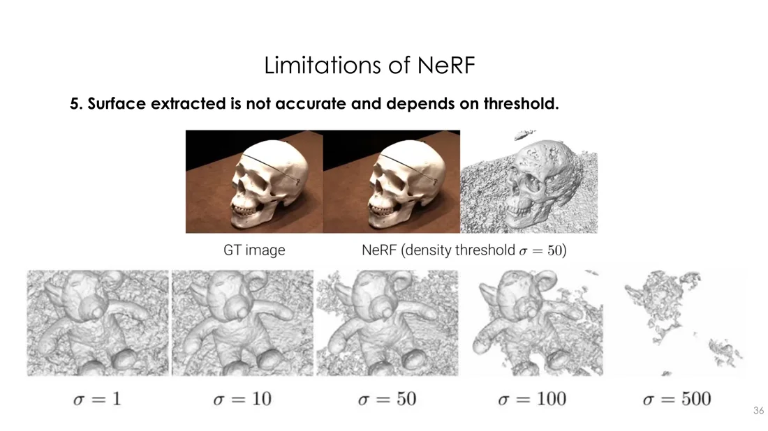
Scene geometry can be approximated using a threshold on the density, or with the expected ray termination depth ${\sum }_i{T}_i{\alpha }_i{t}_i$.

Slide 29: rendered camera path and expected ray termination depth.

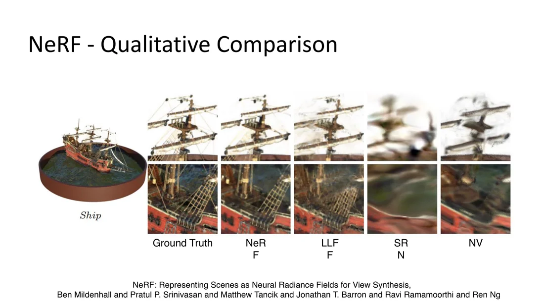
NeRF recovers fine details in geometry and appearance, e.g. the rigging of the Ship, much better than LLFF, SRN and Neural Volumes.

Slide 30: qualitative comparison.

Limitations of NeRF

Slides 31-35

#	Limitation	Addressed by
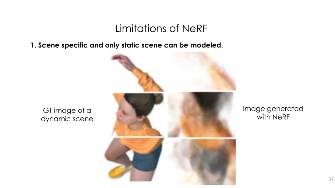
1	Scene-specific, only static scenes can be modeled	D-NeRF
2	No editing and control: the scene is memorized in the network and can’t be modified	Control-NeRF
3	Generalization: scene-specific models, a large number of images needed	Control-NeRF (shared renderer)
4	Expensive training: 10 hours up to a few days; inference is not real time	Instant NGP
5	The extracted surface is not accurate and depends on the density threshold	UniSurf

(NeRF-W addresses a further issue: real internet photos violate NeRF’s assumption of consistent views.)

Slide 31: dynamic scenes fail

Slide 35: surface depends on the threshold σ

Variants of NeRF

D-NeRF: Dynamic Scenes

Slides 36-46

For a dynamic scene there is one more variable: time. We want a radiance field $(x,y,z,\theta ,\varphi ,t)\mapsto (r,g,b,\sigma )$.

Can we learn this directly with NeRF? Adding $t$ as an input gives blurry results: the network can reason about dynamics and shape, but doesn’t learn high-frequency details.

D-NeRF (Pumarola et al., CVPR 2021): split the problem into two stages.

1. A deformation network ${\Psi }_t:(x,y,z,t)\mapsto (\Delta x,\Delta y,\Delta z)$ maps every point at time $t$ into a canonical space (the scene at rest).
2. A canonical network ${\Psi }_x:(x+\Delta x,y+\Delta y,z+\Delta z,\theta ,\varphi )\mapsto (R,G,B,\sigma )$ is a radiance field in the canonical space.

Slide 40: learn a canonical shape and a radiance field in the canonical space.

Slide 42: D-NeRF synthesis with control over time, azimuth and elevation (played 1.5x).

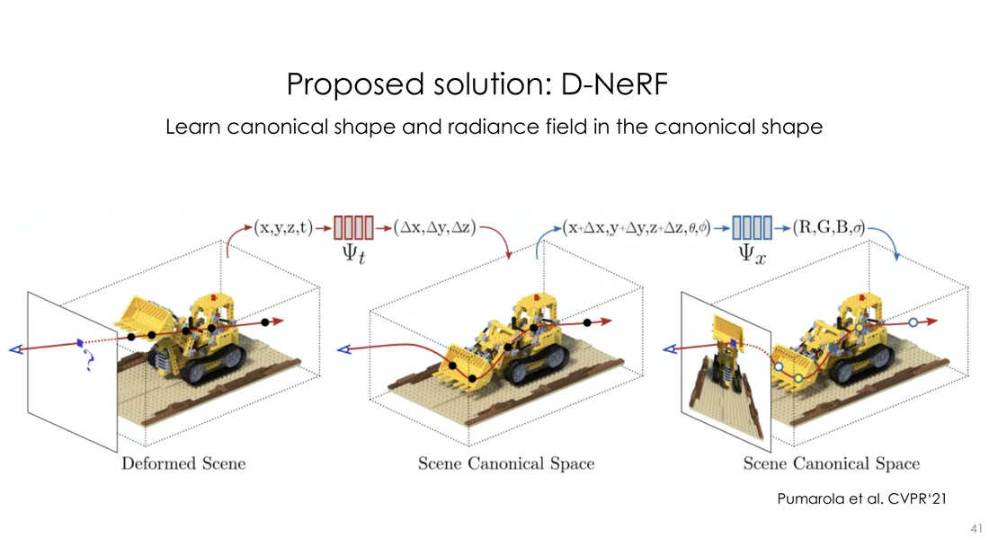
Conclusion: D-NeRF

• Disentangles the time-dependent deformation from the neural rendering network.
• The correspondence between the canonical shape and the deformed shape is defined by $\mathbf{x}+\Delta \mathbf{x}$.
• Time-varying shading effects are modeled: e.g. the floor shadows are warped along time. Points in the shadow of the red ball at $t=0.5$ and $t=1$ map to different regions of the canonical space.

Slide 45: D-NeRF canonical mapping (color-coded as x + Δx).

NeRF-W: NeRF in the Wild

Slides 47-57

NeRF assumes consistent input views: a 3D point seen from the same position and direction in two images has the same intensity. Internet photos violate this with:

• photometric variations (lighting, exposure, white balance)
• transient objects (people, cars, occlusions)

NeRF-W (Martin-Brualla et al., CVPR 2021) introduces per-image appearance embeddings and transient uncertainty fields, which handle lighting changes and occlusions, and performs better on unconstrained Photo Tourism datasets.

Slide 50: NeRF-W architecture. Appearance embedding for the static head, transient embedding and uncertainty β for the transient head.

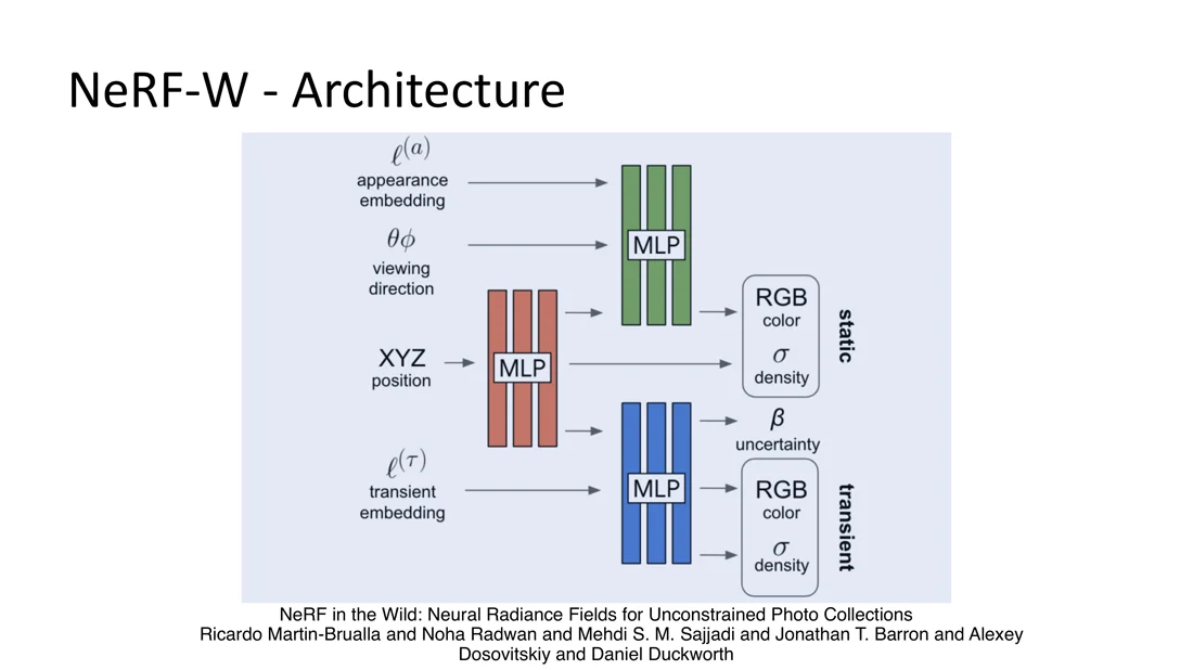
Latent appearance modeling:

• Each image gets an appearance embedding vector ${\ell }_i^{(a)}$, trained with the model.
• The radiance depends on per-image lighting and post-processing, while the geometry stays static.
• Interpolating between two embeddings changes the appearance smoothly without affecting the 3D geometry.

Image-dependent radiance

$${\hat{C}}_i(\mathbf{r})=\mathcal{R}(\mathbf{r},{\mathbf{c}}_i,\sigma )=\sum _{k=1}^{K}T(t_k)\alpha (\sigma (t_k){\delta }_k){\mathbf{c}}_i(t_k),{\mathbf{c}}_i(t)={\text{MLP}}_{{\theta }_2}(\mathbf{z}(t),{\gamma }_{\mathbf{d}}(\mathbf{d}),{\ell }_i^{(a)})$$

Slide 49: interpolating appearance embeddings

Slide 53: Trevi Fountain from internet photos

Transient objects and uncertainty:

• A secondary transient MLP head models moving and occluding objects.
• Both static and transient components (density + color) are rendered, but the transient parts are discarded at test time.
• A per-ray uncertainty $\beta$ down-weights unreliable pixels.

Static + transient compositing

$${\hat{C}}_i(\mathbf{r})=\sum _{k=1}^K{T}_i(t_k)[\alpha (\sigma (t_k){\delta }_k){\mathbf{c}}_i(t_k)+\alpha ({\sigma }_i^{(\tau )}(t_k){\delta }_k){\mathbf{c}}_i^{(\tau )}(t_k)],T_i(t_k)=\exp \left(-\sum _{k^{\prime }=1}^{k-1}[\sigma (t_{k^{\prime }})+{\sigma }_i^{(\tau )}(t_{k^{\prime }})]{\delta }_{k^{\prime }}\right)$$

Static component $\sigma (t),{\mathbf{c}}_i(t)$; transient component ${\sigma }_i^{(\tau )}(t),{\mathbf{c}}_i^{(\tau )}(t)$.

Summary: NeRF-W disentangles lighting from the 3D geometry, which stays consistent, so novel views can be rendered with variable illumination.

Disadvantages: sparse view problems (rarely observed areas like the ground, oblique angles), sensitivity to camera calibration (blurry artifacts from wrong poses), inherited NeRF weaknesses (specular surfaces, high training cost, limited generalization), and transient handling can leave artifacts or mask static scene errors.

Control-NeRF: Scene Manipulation

Slides 58-70

Prior work: the scene is memorized inside the network, which makes compositing and editing hard. Key idea: decouple the scene representation from the neural rendering network.

Control-NeRF (Lazova et al., WACV 2023)

• Hybrid 3D representation: scene-specific 3D feature volumes + a shared neural rendering network.
• Scene-agnostic rendering: one rendering network generalizes across scenes; new scenes are optimized without retraining the whole model.
• Post-hoc scene manipulation: 3D edits (object insertion, deformation, scene mixing) by modifying the feature volumes, without retraining.

Slide 60: decouple scene representation and rendering.

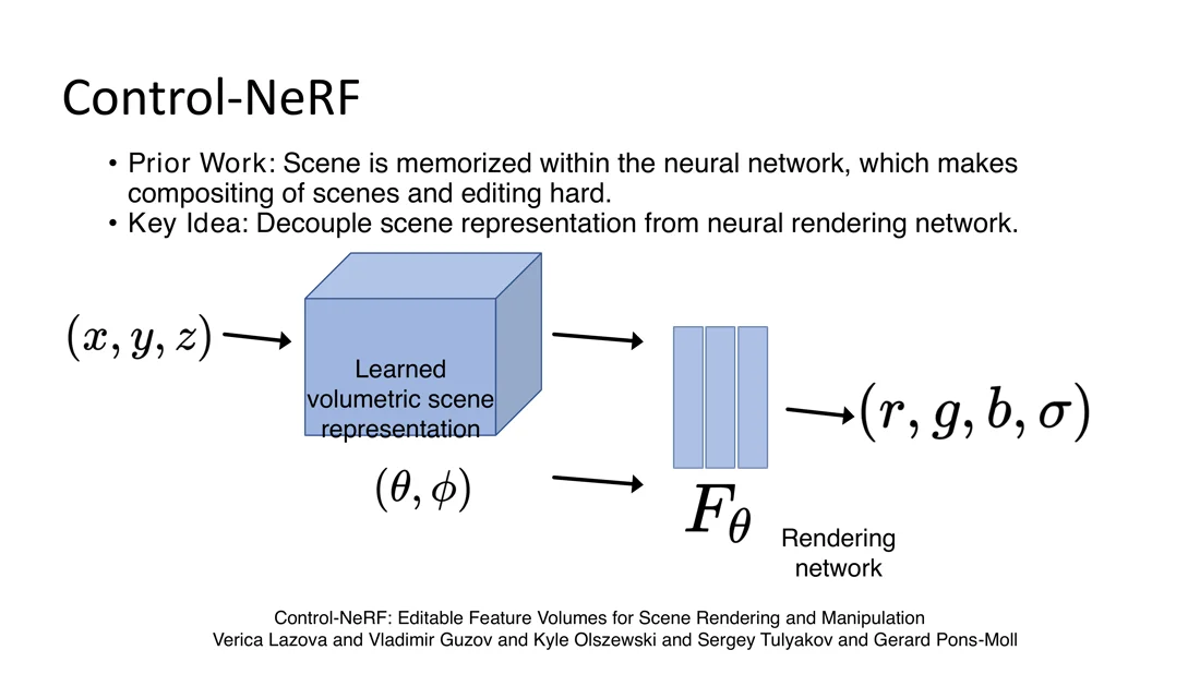
1. Scene representation: given images $\mathcal{I}=\{I_s^i{\}}_{i=1}^{N_s}$ from $M=|\mathcal{S}|$ training scenes, learn a volumetric feature $V_s\in {\mathbb{R}}^{WHDF}$ per scene ($W\times H\times D$ spatial resolution, feature length $F$).
2. Rendering with feature volumes: shoot a ray, query the feature $V_s(\mathbf{p})$ at each point by trilinear interpolation, feed it with the viewing direction to the rendering network $F_{\theta }$, and apply volume rendering.
3. Training and inference: at training time, volumes and rendering network are trained jointly. For a novel scene, the rendering network is fixed and only the scene volume is optimized.

Training details:

• Multi-resolution volume training (coarse to fine): train a $16^3$ volume until convergence, upsample by 2, train again; 4 stages up to $128^3$. Faster training, high-quality synthesis and manipulation.
• Multi-scene training: sample one scene, train for $N$ iterations, save its volume, repeat (loading a new volume every iteration would cost too much GPU memory traffic).
• Generalization to novel scenes: with enough training scenes, the learned radiance function can be reused to optimize new scenes efficiently.

Slide 69: scene editing, inserting a T-rex skeleton into a garden scene.

Instant NGP: Training Speed

Slides 71-83

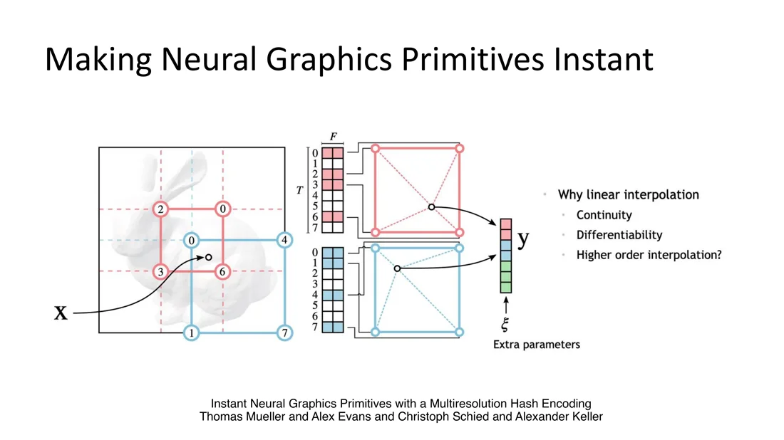
Instant Neural Graphics Primitives with a Multiresolution Hash Encoding (Müller et al., SIGGRAPH 2022):

• train in minutes (instead of days)
• encode high-frequency details more compactly
• render interactively (tens of frames per second)

Three pillars:

Pillar	What it does	Gain
Rendering/training algorithm	task-specific GPU implementation; skips empty space until the surface is hit	10-100x fewer steps than naive dense stepping → fewer network queries
Small neural network	fully fused implementation (the whole MLP in one CUDA kernel)	5-10x faster than TensorFlow
”Good” input encoding	multiresolution hash encoding, trainable together with the network	better speed/quality trade-off, task-agnostic

Slide 73: the three pillars of Instant NGP.

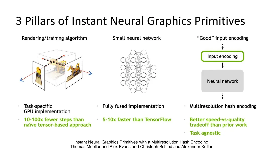
Hash encoding (details in Lecture 6.1 and Hash Encoding):

• Why multi-resolution? Automatic level of detail: low-resolution grids capture global shape, high-resolution grids fine details. The network learns fast at low resolution and refines the details later.
• Hashing: instead of allocating $R^3$ vectors, allocate a much smaller table of size $T$ and map each grid cell to one of the $T$ buckets with a spatial hash. Each bucket stores a learned feature vector. The table is task-agnostic (unlike NGLOD, which needs surface information to build its structure).
• Why linear interpolation? Continuity and differentiability.

Slide 79: multiresolution hash encoding.

Slide 80: instant NeRF training

Slide 82: real-time fly-through, trained in under 5 minutes

Disadvantages (Slide 83):

• Encoding trade-offs: concatenating multiresolution features increases parallelism but also memory and compute.
• Hash function: simple hashing is fast but lacks coherence; better hashes add overhead without clear gains.
• Microstructure artifacts: hash collisions cause grainy noise (e.g. in SDFs), which needs filtering or smoothness priors.
• Future work: differentiable hashing; sparse volumetric data (e.g. clouds) remains open.

UniSurf: Unifying NeRF and Implicit Surfaces

Slides 87-103

The surface extracted from a NeRF is not accurate and depends on the threshold.

Surface rendering (implicit surfaces)	Volume rendering (radiance fields)
✓ high-quality geometry	✗ surface is only approximated
✓ clear surface definition	✓ no mask supervision needed
✗ mask supervision required	✓ high-quality novel views, sharp textures
✗ texture mapping is blurry

UniSurf (Oechsle et al., ICCV 2021) combines the best of both worlds.

Rewrite NeRF’s volume rendering with alpha values:

$$\hat{C}(\mathbf{r})=\sum _{i=1}^N{\alpha }_i\prod _{j=1}^{i-1}(1-{\alpha }_j){\mathbf{c}}_i,{\alpha }_i=1-\exp (-{\sigma }_i{\delta }_i)$$

(The slides write the product up to $i$; it must stop at $i-1$, consistent with $T_i$.)

Key idea of UniSurf

For solid objects, ${\alpha }_i$ corresponds to an occupancy field $o_i\in [0,1]$ at the $i$-th sample:

$${\hat{C}}_v(\mathbf{r})=\sum _{i=1}^N{o}_i\prod _{j<i}(1-o_j){\mathbf{c}}_i$$

Given the occupancy, the same scene can also be rendered with surface rendering (the surface is the level set $o=\tau$).

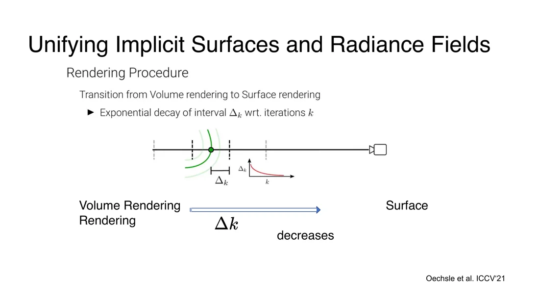
Training schedule: volume rendering in the early stage (optimization without masks), surface rendering in the later stage (level-set surfaces).

Rendering procedure:

1. Find the surface along the ray: uniform sampling + iterative secant method.
2. Define an interval ${\Delta }_k$ around the surface.
3. Volume rendering with occupancies, sampling only inside this interval (fewer points between camera and surface prevents free-space artifacts).

The interval decays exponentially over the iterations $k$. As it shrinks, volume rendering turns into surface rendering:

Theorem (Slide 102)

Volume and surface rendering become equivalent when reducing the interval and increasing the number of samples:

$$\underset{\begin{array}{c}\Delta \to 0\\ N\to \infty \end{array}}{\lim }{\hat{C}}_v(\mathbf{r})={\hat{C}}_s(\mathbf{r})$$

Slide 101: as Δₖ decreases, volume rendering becomes surface rendering.

Slide 103: UniSurf on the DTU MVS dataset.

Upcoming (Slide 86): 3D Gaussian Splatting for real-time radiance field rendering (Kerbl et al., SIGGRAPH 2023) → Lecture 8.

NeRF vs. 3D Gaussian Splatting

For exam task 4. 3DGS is covered in Lecture 8 (symbols of its formula: here); this is the comparison frame.

The two rendering formulas

NeRF:

$$\hat{C}(\mathbf{r})=\sum _{i=1}^N{T}_i{\alpha }_i{\mathbf{c}}_i,{\alpha }_i=1-\exp (-{\sigma }_i{\delta }_i),T_i=\prod _{j=1}^{i-1}(1-{\alpha }_j)$$

3D Gaussian Splatting:

$$C=\sum _{i\in \mathcal{N}}{\mathbf{c}}_i{\alpha }_i\prod _{j=1}^{i-1}(1-{\alpha }_j),{\alpha }_i=o_i\cdot G_i^{2D}(\mathbf{x})$$

($o_i$: learned opacity of Gaussian $i$, $G_i^{2D}$: the projected 2D Gaussian evaluated at the pixel.)

	NeRF	3DGS
Compositing	${\sum }_i{T}_i{\alpha }_i{\mathbf{c}}_i$, $T_i={\prod }_{j<i}(1-{\alpha }_j)$	the same structure
Elements $i$	samples along a ray	Gaussians sorted by depth that overlap the pixel
$\alpha$	computed: $1-\exp (-{\sigma }_i{\delta }_i)$	learned opacity × projected 2D Gaussian
Color	MLP$(\mathbf{x},\mathbf{d})$	spherical harmonics per Gaussian
Representation	implicit (the scene is in the weights $\theta$)	explicit (primitives in space)
Rendering	ray marching, $N$ MLP queries per pixel	rasterization / splatting
Speed	training hours to days, inference not real time	fast training, real-time rendering
Editing	hard (scene in the weights)	easy (move Gaussians directly)
High frequencies	needs positional encoding	small Gaussians, no encoding needed

Intuition

Same compositing formula. They differ in where $\alpha$, $\mathbf{c}$ and the ordering come from, and in how the elements are traversed (marching along rays vs. splatting sorted primitives).

Worked Example: Alpha Compositing

Two samples along a ray

$\sigma =(1,3)$, $\delta =(1,0.5)$.

$${\alpha }_1=1-e^{-1\cdot 1}\approx 0.632,T_1=1,w_1=T_1{\alpha }_1\approx 0.632$$ $${\alpha }_2=1-e^{-3\cdot 0.5}=1-e^{-1.5}\approx 0.777,T_2=1-{\alpha }_1=e^{-1}\approx 0.368,w_2=T_2{\alpha }_2\approx 0.286$$

${\sum }_i{w}_i\approx 0.918\le 1$. The pixel color is $\hat{C}=0.632{\mathbf{c}}_1+0.286{\mathbf{c}}_2$; the remaining $0.082$ is the probability that the ray passes through both samples (background).

Note that sample 2 has the higher density, but gets less weight, because sample 1 already occludes it.

Self-Test

What does NeRF's MLP take as input and give as output?

Answer $(x,y,z)$ and viewing direction $(\theta ,\varphi )$ (with positional encoding). Output: color $(r,g,b)$ and volume density $\sigma$.

Input: 3D position

Write down the continuous volume rendering equation and explain every symbol.

Answer $C(\mathbf{r})={\int }_{t_n}^{t_f}T(t)\sigma (\mathbf{r}(t))\mathbf{c}(\mathbf{r}(t),\mathbf{d})dt$, $T(t)=\exp (-{\int }_{t_n}^t\sigma (\mathbf{r}(s))ds)$, $\mathbf{r}(t)=\mathbf{o}+t\mathbf{d}$. $C$: pixel color; $\mathbf{o},\mathbf{d}$: camera center and ray direction; $t_n,t_f$: near/far bounds; $\sigma$: density; $\mathbf{c}$: view-dependent color; $T$: transmittance (probability of reaching $t$ unblocked).

Why is the transmittance an exponential?

Answer $T(t+dt)=T(t)(1-\sigma (t)dt)$. This gives $T^{\prime }=-T\sigma$, whose solution is $T(t)=\exp (-{\int }_0^t\sigma (u)du)$.

Hits along the ray are independent:

Why is $T(t)\sigma (t)$ a PDF, and what is $1-T(t)$?

Answer $T\sigma$ = "reach $t$" × "stop at $t$" = density of the stopping position. $1-T(t)$ is the CDF: the probability of having hit something before $t$.

Write down the discrete NeRF rendering formula and explain ${\alpha }_i$, $T_i$, ${\delta }_i$, $t_i$.

Answer $\hat{C}={\sum }_i{T}_i(1-e^{-{\sigma }_i{\delta }_i}){\mathbf{c}}_i$. ${\alpha }_i=1-e^{-{\sigma }_i{\delta }_i}$: probability to stop within segment $i$ (computed, not learned). $T_i=\exp (-{\sum }_{j<i}{\sigma }_j{\delta }_j)={\prod }_{j<i}(1-{\alpha }_j)$: probability to reach sample $i$. ${\delta }_i=t_{i+1}-t_i$. $t_i$: random position inside the $i$-th of $N$ evenly spaced bins.

How is NeRF trained? What happens at inference time?

Answer $(\mathbf{c},\sigma )$, volume rendering gives the pixel color, minimize the squared error to the ground-truth pixel, backpropagate. Inference: render rays from a new camera pose with the trained MLP.

Training: rays from posed photos, samples along the rays, MLP gives

Why does NeRF need positional encoding?

Answer $\gamma (p)=(\sin (2^k\pi p),\cos (2^k\pi p){)}_{k=0}^{L-1}$ increase the spectrum.

Coordinate MLPs are biased towards low frequencies (limited NTK bandwidth), so results are blurry. Fourier features

Name five limitations of NeRF and a variant that addresses each.

Answer

Static scenes only → D-NeRF. No editing → Control-NeRF. No generalization, many images → Control-NeRF (shared renderer). Slow training/inference → Instant NGP. Inaccurate, threshold-dependent surfaces → UniSurf.

How does D-NeRF model dynamic scenes?

Answer ${\Psi }_t(\mathbf{x},t)=\Delta \mathbf{x}$ maps each point to a canonical space; a canonical radiance field ${\Psi }_x(\mathbf{x}+\Delta \mathbf{x},\mathbf{d})$ gives color and density. This disentangles deformation from rendering.

A deformation network

How does NeRF-W handle internet photos?

Answer $\beta$ models moving objects and occluders; it is discarded at test time.

Per-image appearance embeddings (lighting, exposure) change the color but not the geometry. A transient head with uncertainty

What is the key idea of Control-NeRF?

Answer

Decouple the scene (per-scene feature volumes) from a shared rendering network. For new scenes, only the volume is optimized. Editing = manipulating the feature volumes.

What are the similarities and differences between NeRF and 3DGS rendering?

Answer ${\sum }_i{T}_i{\alpha }_i{\mathbf{c}}_i$ with $T_i={\prod }_{j<i}(1-{\alpha }_j)$. NeRF: implicit MLP, $\alpha$ computed from $\sigma$ and $\delta$, ray marching, slow. 3DGS: explicit Gaussians, $\alpha$ = learned opacity × 2D Gaussian, depth-sorted rasterization, real time, editable.

Same alpha compositing

Related

• Previous: Lecture 6.2: Point Cloud Processing · Next: Lecture 8: 3D Gaussian Splatting · Course: Overview
• Concepts: Gaussian Splatting, Volume Rendering, Positional Encoding, Neural Field, Hash Encoding, Inverse Rendering, Implicit and Explicit Representations, Occupancy Field
• NeRF needs camera poses, usually from COLMAP. 3D Gaussian Splatting follows in Lecture 8.