Lecture 9: Learning-Based 3D Reconstruction

TL;DR

1. Classical SfM (COLMAP) is a long pipeline of sub-problems, each solved imperfectly, with repeated bundle adjustment: accurate when it works, but brittle and slow.
2. DUSt3R (CVPR 2024) shifts the paradigm: a single network takes two unposed, uncalibrated images and directly regresses two point maps, both in camera 1’s frame.
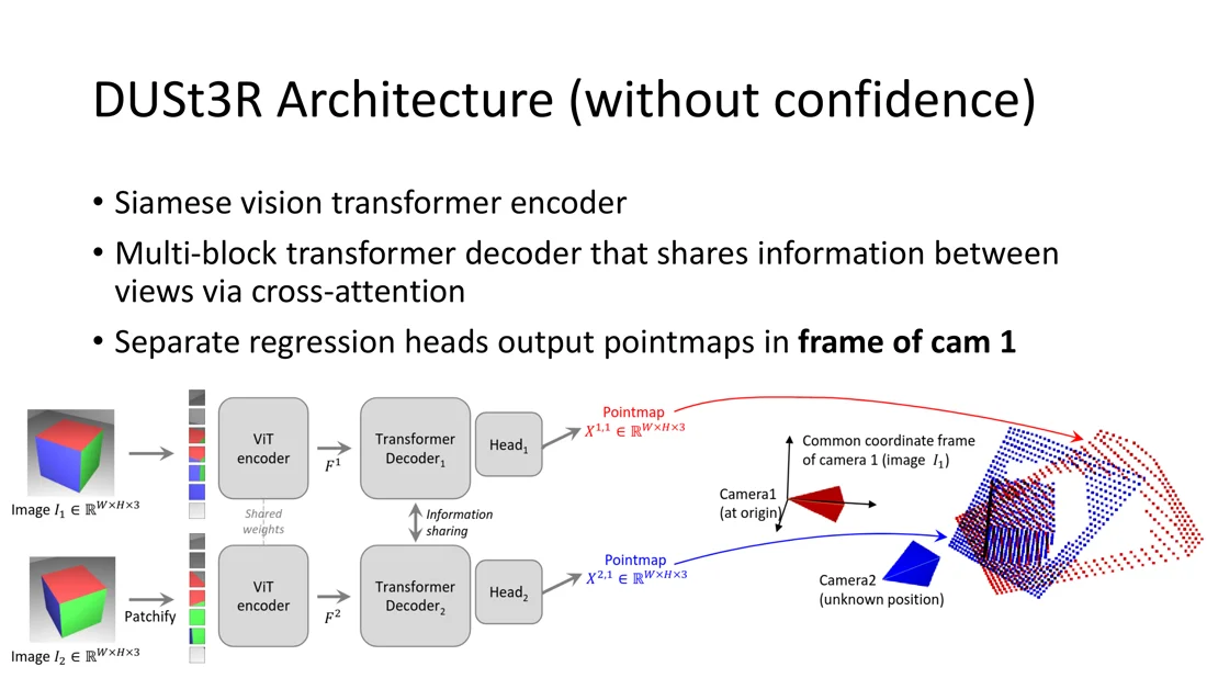
3. A point map $X\in {\mathbb{R}}^{W\times H\times 3}$ is a dense, pixel-aligned point cloud: a 1-to-1 mapping between pixels and 3D points. Depth, correspondences, focal length and relative pose can all be read from it.
4. Training: a scale-normalized 3D regression loss, weighted by a learned confidence $C=1+e^{\tilde{C}}$ with a $-\alpha \log C$ penalty. More than 2 views need global alignment of $O(N^2)$ pairs.
5. MASt3R adds metric point maps and a matching head; MASt3R-SfM makes multi-view sparse; Fast3R and VGGT reconstruct many views in one forward pass (VGGT: alternating frame/global attention, predicts cameras, depth, point maps and tracks).
6. Point-map models also initialize or predict 3D Gaussians from few views (InstantSplat, Splatt3R).

Exam relevance

In exam task 3 (point cloud → mesh), a sub-question asked for the difference between a point cloud and a point map. See Point Maps. Also: the DUSt3R input/output and architecture, and what can be derived from point maps.

flowchart LR
  A["Classical SfM<br/>COLMAP"] --> B["Classical +<br/>learned components<br/>SuperPoint, SuperGlue, DISK"] --> C["End-to-end<br/>learnable SfM<br/>DeepSfM, VGGSfM"] --> D["Learned +<br/>global alignment<br/>DUSt3R, MASt3R"] --> E["Single<br/>forward pass<br/>VGGT"]

From left (traditional, optimization-based: epipolar geometry, pose estimation, triangulation, bundle adjustment) to right (modern, learning-based: feature matching, monocular depth, cross-view attention).

From Classical to Learned Reconstruction

Reconstruction: The Core of 3D

Slides 2-5

3D reconstruction has been a key research problem for over 50 years: recover a point cloud and camera poses from several unconstrained images. In Lecture 3 we saw the traditional methods (SfM and MVS): unstructured images → scene graph → sparse model (SfM) → dense model (MVS).

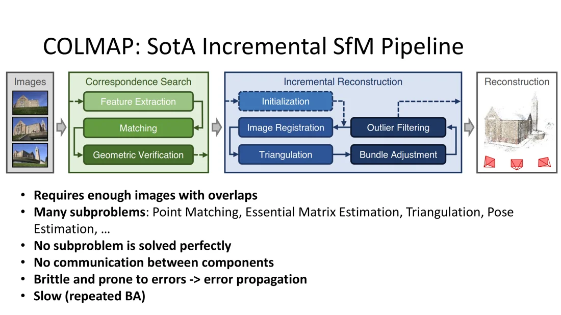
COLMAP, the state-of-the-art incremental SfM pipeline, builds on decades of engineering. When it works, its reconstructions are very good. But:

• it requires enough images with overlap
• it has many sub-problems: point matching, essential matrix estimation, triangulation, pose estimation, …
• no sub-problem is solved perfectly
• there is no communication between components
• it is brittle and prone to errors → error propagation (the pipeline is only as good as its weakest component)
• it is slow: bundle adjustment is repeated every time a new image is registered (test-time optimization)

Slide 4: COLMAP, the state-of-the-art incremental SfM pipeline.

Traditional Pipelines with Learned Components

Slides 6-9

Recent trend: replace certain parts of the SfM pipeline with learned modules: SuperPoint (features), SuperGlue (matching), DISK (features), LevelS²fM (neural bundle adjustment). They make single components more robust, but the general problem remains.

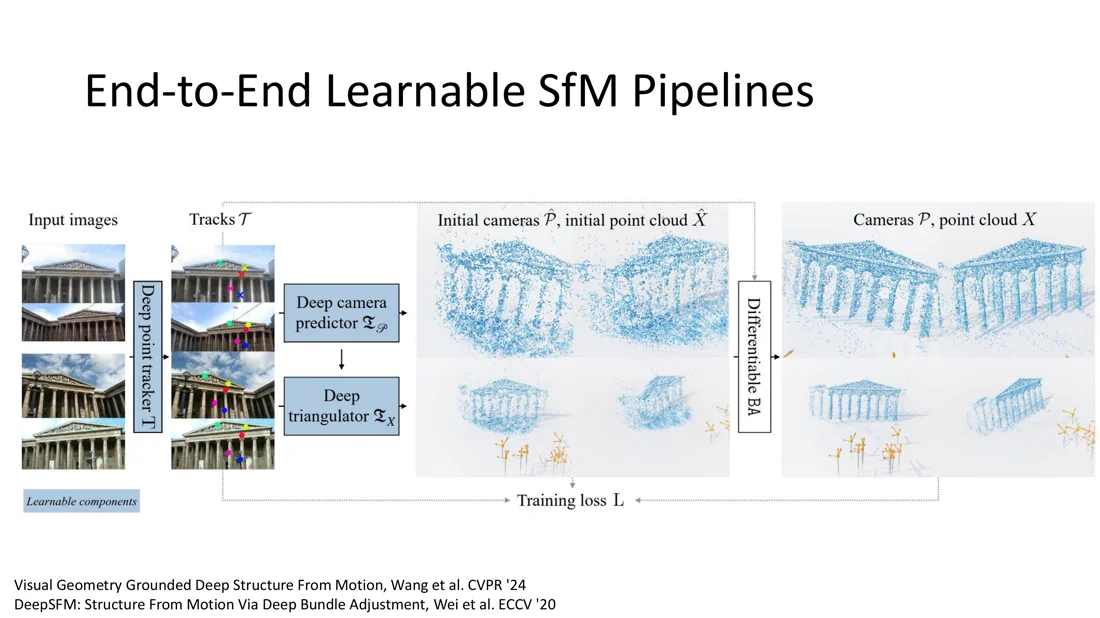
End-to-end learnable SfM pipelines (DeepSfM, ECCV 2020; VGGSfM, CVPR 2024) replace every component by a differentiable, learnable module and train end-to-end. But they still follow the classical structure (camera pose estimation, triangulation, BA), so the same problems remain.

Slide 8: an end-to-end learnable SfM pipeline (VGGSfM).

What would be even further to the right on the spectrum?

Answer directly outputs the 3D points. That is DUSt3R.

Leave the keypoint → pose → triangulation structure behind: a network that takes two (or more) images and

DUSt3R

DUSt3R: Shifting the Paradigm

Slide 10

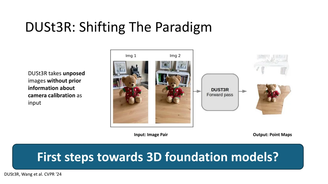
DUSt3R (Wang et al., CVPR 2024) takes unposed images without prior information about the camera calibration and directly regresses 3D points in one forward pass. First steps towards 3D foundation models?

Slide 10: image pair in, point maps out.

Point Maps

Slide 11

Point map

• a dense, pixel-aligned 3D point cloud: $\mathbf{X}\in {\mathbb{R}}^{W\times H\times 3}$
• forms a 1-to-1 mapping between image pixels and 3D scene points: ${\mathbf{I}}_{i,j}\leftrightarrow {\mathbf{X}}_{i,j}$
• more structured than a point cloud
• easy conversion: point map ↔ depth map

Slide 11: every pixel of the image has its 3D point.

	Point cloud	Point map	Depth map
Structure	unordered set of $N$ points	image grid $W\times H$, one 3D point per pixel	image grid $W\times H$, one value per pixel
Stored	$(x,y,z)$ per point	$(x,y,z)$ per pixel	only $z$ per pixel
Pixel correspondence	none	1-to-1 pixel ↔ point	1-to-1, but needs intrinsics to get 3D
Coordinate frame	any	a chosen camera frame (DUSt3R: camera 1)	its own camera
Density	sparse or dense	dense	dense

Intuition

A point map is a point cloud that keeps the image structure. Because each pixel knows its 3D point, the 2D neighborhood tells you which points belong together, and the 2D-3D correspondence is given for free. That is why depth, focal length, pixel correspondences and camera pose can all be derived from it.

DUSt3R Task and Architecture

Slides 12-14

Task

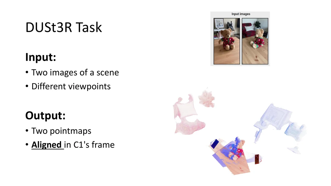
Input: two images of a scene from different viewpoints. Output: two point maps $X^{1,1},X^{2,1}\in {\mathbb{R}}^{W\times H\times 3}$, aligned in camera 1’s frame.

Notation: $X^{i,j}$ is the point map of image $i$ in the frame of camera $j$.

Slide 12: the DUSt3R task.

Architecture (without confidence):

1. A Siamese ViT encoder (shared weights) patchifies and encodes both images → tokens $F^1,F^2$.
2. A multi-block transformer decoder shares information between the views via cross-attention.
3. Separate regression heads output the point maps, both in the frame of camera 1.

Slide 13: DUSt3R architecture.

Decoder blocks (from CroCo, Weinzaepfel et al., NeurIPS 2022): 8 blocks in series. In each block:

• self-attention across all patches of the same image
• cross-attention to the patches of the other image (information sharing)
• an MLP, then on to the next block

Each image has its own decoder branch (the slide shows one).

Slide 14: DUSt3R decoder blocks.

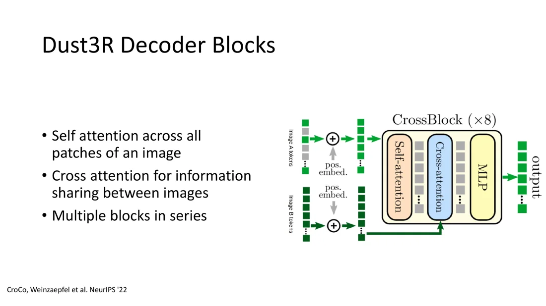
(See Attention for self- and cross-attention.)

Training Objective

Slide 15

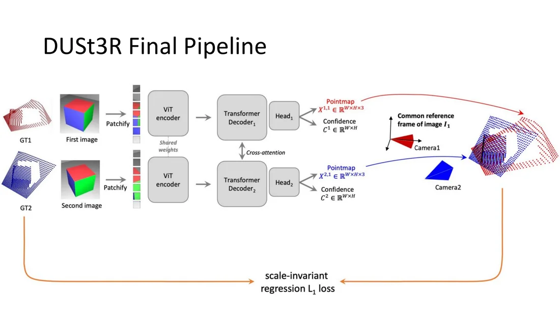
Minimize the deviation of the predicted point maps from the ground-truth point maps (easily obtained from ground-truth depth maps). Prediction and ground truth can differ in scale, so both are normalized by the average distance of the points to the origin:

3D regression loss

$${\ell }_{regr}(v,i)=\Vert \frac{1}{z}{X}_i^{v,1}-\frac{1}{\bar{z}}{\bar{X}}_i^{v,1}\Vert ,z=\frac{1}{|{\mathcal{D}}^1|+|{\mathcal{D}}^2|}\sum _{v\in \{1,2\}}\sum _{i\in {\mathcal{D}}^v}\Vert X_i^v\Vert$$

$v\in \{1,2\}$: view; $i$: image pixel (with valid ground truth, ${\mathcal{D}}^v$); $X_i^{v,1}$: predicted point; ${\bar{X}}_i^{v,1}$: ground-truth point; $z,\bar{z}$: normalizing factors.

Confidence-Aware Training

Slides 16-19

Dealing with ambiguous points: what is the ground-truth position of the sky, or of a ship inside a glass bottle? Even humans are not confident. So the heads regress not only the point maps but also a per-pixel confidence score $C^{1,1},C^{2,1}\in {\mathbb{R}}^{W\times H}$. How do we train it without ground truth for the confidence?

Confidence-aware loss (Slide 18)

$${\mathcal{L}}_{conf}=\sum _{v\in \{1,2\}}\sum _{i\in {\mathcal{D}}^v}{C}_i^v{\ell }_{regr}(v,i)-\alpha \log C_i^v,C_i^v=1+\exp {\tilde{C}}_i^v$$

$C_i^v$: confidence of pixel $i$ in view $v$; ${\ell }_{regr}$: regression loss; $\alpha$: regularization weight (penalty for uncertainty); ${\tilde{C}}_i^v$: the network output.

Intuition

The loss is minimized by a low regression error and a high confidence (then $-\alpha \log C$ is negative). For ambiguous points it is better to lower the confidence (the first term shrinks) and pay the price $\alpha \log C$. Forcing $C>1$ (via $1+e^{\tilde{C}}$) makes the model extrapolate in uncertain areas (e.g. regions visible in only one image) instead of outputting arbitrary points with zero confidence. It also reduces the effect of noisy labels (glass and thin structures in laser scans, registration errors).

Slide 19: the final DUSt3R pipeline, trained with a scale-invariant regression loss.

Slide 20: reconstruction + confidence maps.

Robustness

Slides 21-23

Even with drastic viewpoint changes (e.g. opposite views of a motorbike) or no overlap at all between the two images, DUSt3R often regresses a sensible 3D structure. It has learned a very generic 3D prior.

Slide 21: heavy viewpoint changes

Slide 23: no overlap

Multi-View Reconstruction: Global Alignment

Slides 24-26

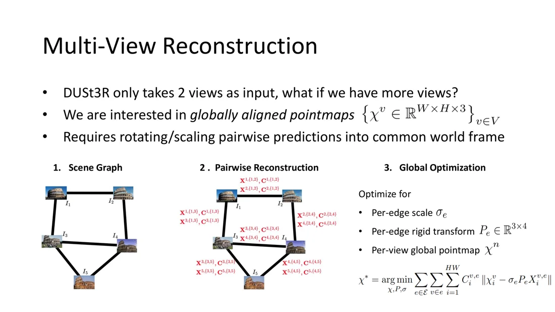
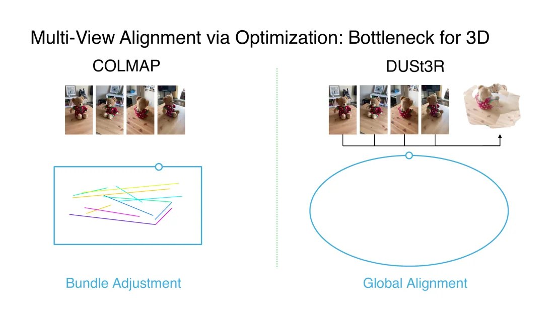
DUSt3R only takes 2 views. With more views we want globally aligned point maps $\{{\chi }^v\in {\mathbb{R}}^{W\times H\times 3}{\}}_{v\in \mathcal{V}}$, which requires rotating and scaling the pairwise predictions into a common world frame:

1. Scene graph: nodes = images, edges = pairs that share visual content (from off-the-shelf retrieval, from DUSt3R’s average confidence, or simply the complete graph).
2. Pairwise reconstruction: run DUSt3R on every edge → point maps $X^{v,e}$ and confidences $C^{v,e}$.
3. Global optimization:

Global alignment

$${\chi }^{\ast }=\arg \underset{\chi ,P,\sigma }{\min }\sum _{e\in \mathcal{E}}\sum _{v\in e}\sum _{i=1}^{HW}{C}_i^{v,e}\Vert {\chi }_i^v-{\sigma }_e{P}_e{X}_i^{v,e}\Vert$$

Optimize for a per-edge scale ${\sigma }_e$, a per-edge rigid transform $P_e\in {\mathbb{R}}^{3\times 4}$, and a per-view global point map ${\chi }^v$.

Slide 24: multi-view reconstruction with DUSt3R.

Global alignment is not bundle adjustment

It minimizes a 3D error between point maps, not a 2D reprojection error. It is run with gradient descent, only once (not after every added view), and converges in a few hundred steps (seconds). But it has to handle $O(N^2)$ point maps, which is very memory-intensive.

Downstream Tasks from Point Maps

Slides 27-34

DUSt3R is trained only for 2-view reconstruction, but the point map is expressive enough for a whole family of 3D tasks: camera calibration, depth estimation (monocular, multi-view), pixel correspondences, camera pose estimation (relative, multi-view, visual localization), dense 3D reconstruction.

Slide 30: towards 3D foundation models.

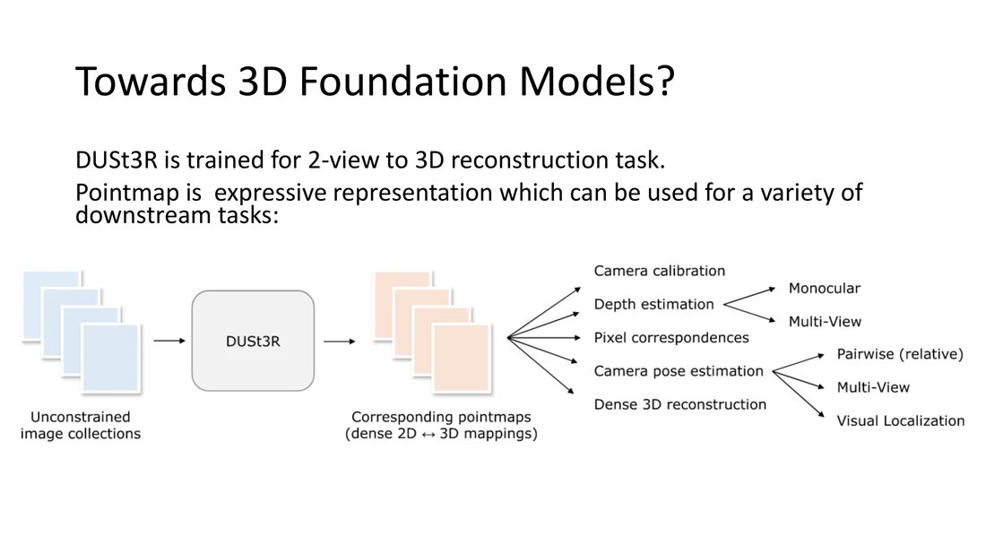
Monocular depth estimation: feed the same image twice; the depth is the $z$ coordinate of the 3D point. Although it was not trained for this, DUSt3R outperforms self-supervised methods and is on par with supervised ones (zero-shot).

Pixel correspondences: image correspondence search becomes a 3D correspondence search, e.g. with mutual nearest neighbors:

Correspondences

$${\mathcal{M}}_{1,2}=\{(i,j)\mid i={\text{NN}}_1^{1,2}(j)\text{ and }j={\text{NN}}_1^{2,1}(i)\},{\text{NN}}_k^{n,m}(i)=\arg \underset{j\in \{0,\dots ,WH\}}{\min }\Vert X_j^{n,k}-X_i^{m,k}\Vert$$

Focal length: assume a centered principal point ($i^{\prime }=i-\frac{W}{2}$, $j^{\prime }=j-\frac{H}{2}$), then minimize a confidence-aware reprojection loss (solved with the Weiszfeld algorithm in a few iterations):

Focal length from a point map

$$f_1^{\ast }=\arg \underset{f_1}{\min }\sum _{i=0}^W\sum _{j=0}^H{C}_{i,j}^{1,1}\Vert (i^{\prime },j^{\prime })-f_1\frac{(X_{i,j,0}^{1,1},X_{i,j,1}^{1,1})}{X_{i,j,2}^{1,1}}\Vert$$

This is the pinhole projection $x=f\frac{X}{Z}$, solved for $f$.

Relative camera pose:

1. Procrustes: feed both ordered pairs $(I_1,I_2)$ and $(I_2,I_1)$, align the point maps with Procrustes, derive the relative pose. Not very robust.
2. PnP + RANSAC: possible because the point map gives 2D-3D correspondences; more robust.

MVS benchmark on DTU: learning-based methods have overtaken handcrafted ones, but DUSt3R cannot compete in 3D accuracy, because (1) regression is less precise than sub-pixel triangulation, (2) it does not use the ground-truth camera poses, (3) it is zero-shot (the others trained on DTU, whose robot always uses the same camera poses).

DUSt3R summary (Slide 35)

• ✓ very robust, even to extreme view changes
• ✓ a simpler end-to-end learnable pipeline → less error accumulation
• ✓ requires only 2 views
• ✗ more views need global alignment: inefficient pairwise processing of $O(N^2)$ pairs, information sharing only between two images at a time, faster than BA but not instant, memory-intensive (out of memory on an 80 GB A100 with 48 views)
• ✗ cannot compete in 3D reconstruction accuracy
• ✓ competitive in many other tasks (depth, pose estimation)

Beyond DUSt3R: 3R Models

Since DUSt3R there has been an explosion of “3R” models: MASt3R, Fast3R, CUT3R, Spann3R, MonST3R, Easi3R, SLAM3R, …

MASt3R: DUSt3R + Matching

Slides 37-40

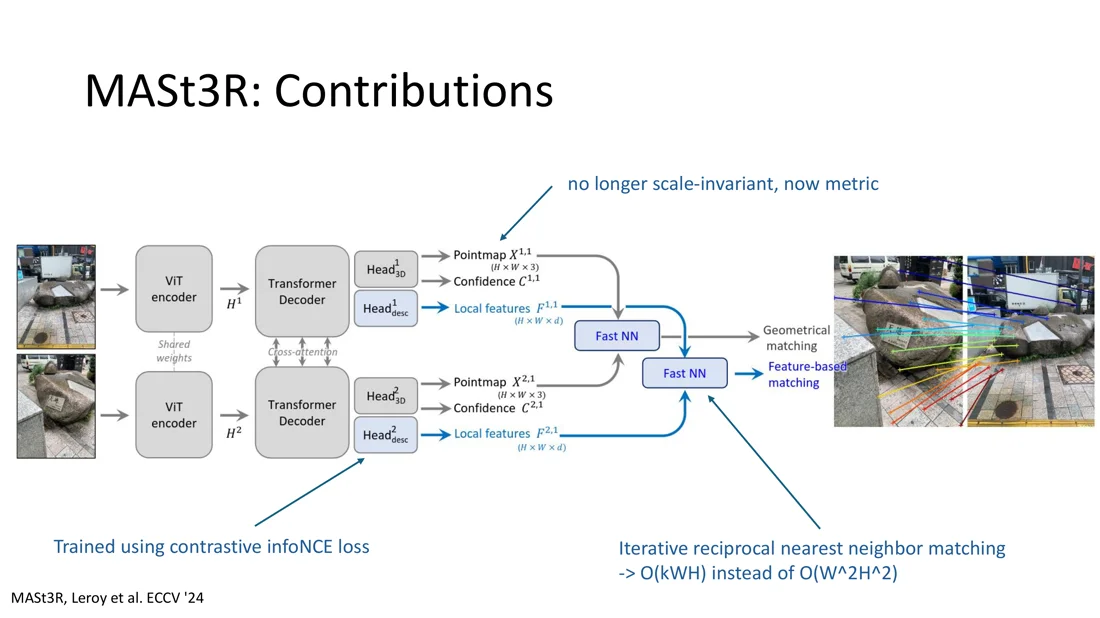
MASt3R (Leroy et al., ECCV 2024): DUSt3R with an additional head that produces per-pixel features for correspondence matching. It inherits DUSt3R’s robustness to heavy viewpoint changes.

• point maps are no longer scale-invariant, but metric (the normalization in the loss is removed)
• the feature head is trained with a contrastive InfoNCE loss (features of matching pixels are pulled together, non-matches pushed apart; supervised by ground-truth matches)
• fast iterative reciprocal nearest-neighbor matching: $O(kWH)$ instead of $O(W^2{H}^2)$ ($k$ = number of matches)

Slide 38: MASt3R contributions.

MVS with MASt3R: forward passes give 2D-2D correspondences, which are triangulated with the ground-truth cameras. No costly global alignment needed. Triangulation outperforms regression: MASt3R beats DUSt3R and is competitive with learning-based MVS methods, without using camera poses for matching and without seeing the DTU setup in training. (The lecturer notes that the comparison is not entirely fair, since MASt3R uses ground-truth cameras for triangulation.)

MASt3R summary

Metric point maps, a feature head for matching, fast reciprocal NN matching; retains DUSt3R’s robustness plus the strengths of pixel matching; outperforms DUSt3R on many tasks. Still pairwise: multiple images still need memory-intensive global alignment.

Efficiently Dealing with More Views: MASt3R-SfM

Slides 42-46

DUSt3R and MASt3R are 2-view models. For $N$ views: an almost complete scene graph with $O(N^2)$ edges → $O(N^2)$ forward passes → global alignment over $O(N^2)$ point maps. Infeasible for large $N$.

MASt3R-SfM (Duisterhof et al., 2024) makes it sparse:

• all images go through the frozen MASt3R encoder once; a sparse scene graph with only $O(N)$ edges is built from the image features
• only these pairs go through the decoder → point maps and matches
• coarse alignment: minimize a 3D loss only for matching points
• refinement: minimize the 2D reprojection loss (like BA)

Coarse alignment in MASt3R-SfM

Canonical point map per image (averaging over its edges):

$${\tilde{X}}_{i,j}^n=\frac{{\sum }_{e\in {\mathcal{E}}^n}{C}_{i,j}^{n,e}{X}_{i,j}^{n,e}}{{\sum }_{e\in {\mathcal{E}}^n}{C}_{i,j}^{n,e}}$$

Estimate the intrinsics $K_n$ via the focal length, then find rigid transforms and scales:

$$\underset{\sigma ,P}{\min }\sum _{(n,m)\in \mathcal{E}}\sum _{i\in {\mathcal{M}}^{n,m}}{C}_i{\Vert {\chi }_i^n-{\chi }_i^m\Vert }^{1.5},{\chi }_i^n=\frac{1}{{\sigma }_n}{P}_n^{-1}{K}_n^{-1}{Z}_i^n\left[\begin{array}{c}u\\ v\\ 1\end{array}\right]$$

The sum only runs over pixel correspondences ${\mathcal{M}}^{n,m}$, not over full point maps.

Optimization is often the bottleneck for 3D vision: it is time-consuming, poorly compatible with deep learning (not plug-and-play, often non-differentiable), and complex (“scary for non-experts”). Can we do without optimization, in one single forward pass?

Slide 43: multi-view alignment via optimization, the bottleneck for 3D.

Fast3R: Many Views in One Pass

Slides 48-51

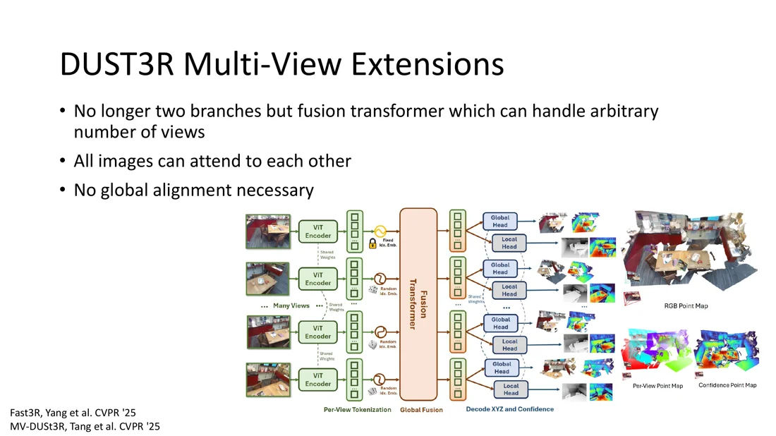
Fast3R (Yang et al., CVPR 2025) and MV-DUSt3R (Tang et al., CVPR 2025) extend DUSt3R to many views:

• no longer two branches, but a fusion transformer that handles an arbitrary number of views
• all images can attend to each other (all-to-all self-attention over the concatenated patch tokens)
• no global alignment necessary

Compared to DUSt3R: much faster and more memory-efficient (DUSt3R runs out of memory at 48 views, Fast3R handles 1500), with information sharing between all views. But on camera pose estimation it is worse than MASt3R: the efficiency comes at a price.

Slide 49: DUSt3R multi-view extensions (Fast3R).

VGGT: Reconstruction in One Go

Slides 52-68

VGGT, Visual Geometry Grounded Transformer (Wang et al., CVPR 2025, Best Paper Award): given a set of images, a single neural network recovers cameras, depth maps, point maps and correspondences (tracks), in one forward pass.

VGGT architecture

1. DINO patchifies every image into tokens.
2. A randomly initialized camera token is added per frame to aggregate camera information.
3. All tokens are concatenated and passed through alternating attention ($L$ times): global self-attention over all frames, then frame-wise self-attention within each frame.
4. A small transformer (camera head) decodes the camera tokens into camera parameters; a DPT head turns the image tokens into dense outputs (depth maps, point maps, tracks).

Slide 54: the VGG Transformer.

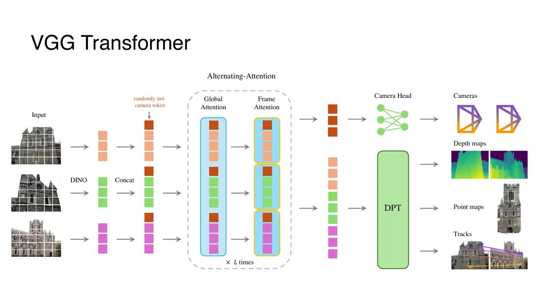
Why an over-parameterized output? DUSt3R extracts depth maps, cameras and matches from the point map. VGGT predicts all of them “independently”. These redundant predictions bring substantial performance gains during training, and at inference, combining estimates (e.g. depth + cameras → points) often outperforms the direct point-map branch.

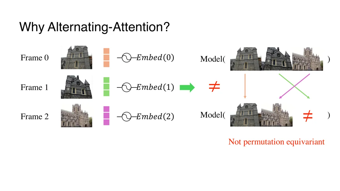
Why alternating attention?

• Global attention ensures scene-level coherence across frames.
• Frame-wise attention replaces a frame index embedding:
  • permutation equivariance: with an embedding $\text{Embed}(1)\ne \text{Embed}(2)$, swapping two input frames would change the reconstruction, although the building is still the same
  • flexible input length: at test time the model would meet embeddings like $\text{Embed}(842)$ that it never saw in training
  • frame-wise attention lets the model learn which tokens belong to the same frame, without an explicit index

Slide 57: with frame index embeddings, the model is not permutation equivariant.

Training and data: trained with 2 to 24 frames, used at inference with 1 to 300+ frames. 17 public datasets: 59% synthetic, 24% captured (e.g. LiDAR), 18% SfM-annotated. More synthetic data → more accuracy; more of the other two → better generalization.

Slide 61: VGGT on out-of-domain inputs (played 1.5x).

Results:

• Accurate: better camera pose estimation (RealEstate10K AUC@30: 85.3) than optimization-based methods and concurrent networks, in a single feed-forward run. Multi-view depth without ground-truth cameras is competitive with MVS methods that need them (camera regression during training makes the model encode camera information implicitly).
• Fast: about 0.2 s instead of about 10 s for optimization-based methods (~50× faster).
• Scaling: memory grows roughly linearly with the number of frames, runtime about $O(N^{1.5})$.
• Zero-shot monocular depth: as good as specialized models like Depth Anything v2, although VGGT was never trained for single-view input.

Slide 67: zero-shot monocular depth with VGGT.

VGGT is general, seamless and practical

• general: diverse images, a single to hundreds of views
• seamless: just a neural network, standard components
• practical: fast and accurate, addresses all core 3D tasks

Novel View Synthesis from Sparse Images

Slides 70-75

Point-map models are binocular and need alignment for many views, which we saw as a downside. But it is also a strength: they are very robust with only a few views, which makes them a perfect fit for sparse-view applications.

Slide 71: scenes reconstructed as 3D Gaussians from only 3 views.

Original 3DGS	InstantSplat (Fan et al., 2024)
assumes known camera parameters	unknown cameras
requires lots of views	few views
sparse initialization from SfM	dense initialization from MASt3R point maps
adaptive density control necessary	joint pose and Gaussian optimization instead

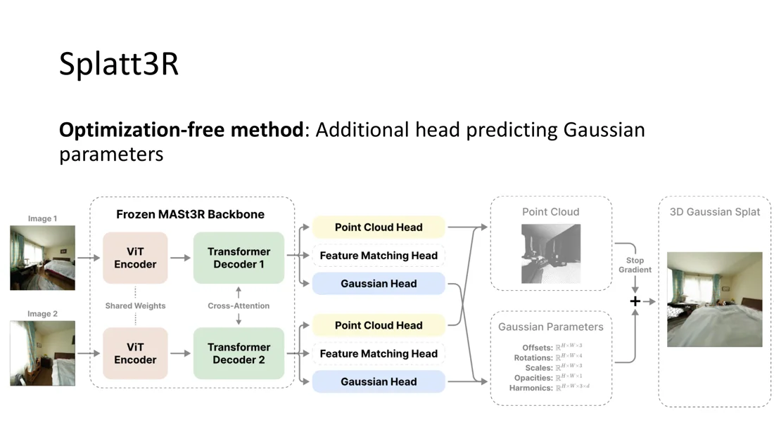
Splatt3R: an optimization-free method. A frozen MASt3R backbone gets an additional Gaussian head that predicts the Gaussian parameters (offsets, rotations, scales, opacities, harmonics) directly from two uncalibrated images. The DUSt3R/MASt3R architecture adapts easily to new tasks: add a head, train on task-specific data.

Slide 74: Splatt3R.

Slide 75: uncalibrated image pair → inference → 3D Gaussian splat → novel renderings.

(3DGS basics: Lecture 8.)

Summary

Slides 76-77

• Traditional 3D reconstruction pipelines are overtaken by learning-based methods.
• DUSt3R shifted the paradigm towards direct point-map regression from unposed images.
• Very robust and versatile; outperforms task-specific methods in classical 3D tasks.
• Sparked a wave of 3R methods for all kinds of applications.
• VGGT: an optimization-free feed-forward network outperforming the state of the art.

Not covered: 3R models for videos and dynamic scenes (Spann3R, MonST3R, DAS3R, CUT3R, Easi3R).

Method	Views	Output	Multi-view	Key idea
COLMAP	many	poses + sparse points	incremental BA	classical pipeline
DUSt3R	2	2 point maps (+ confidence) in cam 1 frame, scale-invariant	global alignment, $O(N^2)$	direct regression, cross-attention
MASt3R	2	metric point maps + matching features	global alignment / MASt3R-SfM (sparse, $O(N)$)	matching head, InfoNCE
Fast3R	many	point maps	one pass	fusion transformer, all-to-all attention
VGGT	1 to 300+	cameras, depth, point maps, tracks	one pass	alternating attention, camera tokens

Extra: Feat2GS

Slides 78-86

Feat2GS: Probing Visual Foundation Models with Gaussian Splatting (Chen et al., CVPR 2025). How well do visual foundation models (DINO, CLIP, MAE, SAM, DUSt3R, MASt3R, RADIO, …) understand the 3D world?

• Previous 3D probing regresses depth or normals from the features and needs 3D ground truth, which limits the data. Feat2GS uses novel view synthesis as the proxy task: only 2D images are needed.
• A shallow 2-layer MLP (shared across views) reads out 3D Gaussian parameters from the features (DUSt3R initialization), trained with a photometric loss.
• Geometry (position, opacity, covariance) and texture (SH coefficients) are probed separately.
• Findings: 3D metrics and 2D (novel view) metrics are well aligned. Foundation models capture geometry well, but struggle with texture, even worse than raw image values.

Slide 82: probing geometry and texture separately.

Self-Test

What are the problems of COLMAP-style pipelines?

Answer

Need enough overlapping images; many sub-problems, none solved perfectly; no communication between components; brittle, errors propagate; slow because bundle adjustment is repeated for every added view.

What are the input and output of DUSt3R?

Answer $X^{1,1},X^{2,1}\in {\mathbb{R}}^{W\times H\times 3}$, both in camera 1's frame, plus confidence maps.

Input: two unposed, uncalibrated images. Output: two point maps

What is the difference between a point cloud and a point map?

Answer $W\times H\times 3$: every pixel has its 3D point (1-to-1), in a given camera frame. It keeps the image structure, so depth, correspondences, focal length and pose can be derived.

A point cloud is an unordered set of 3D points. A point map is a dense, pixel-aligned point cloud

Describe the DUSt3R architecture.

Answer

Siamese ViT encoder with shared weights; two transformer decoders (8 blocks of self-attention within an image, cross-attention to the other image, MLP); two regression heads outputting point maps and confidences in camera 1’s frame.

Write down the confidence-aware loss and explain why $C=1+e^{\tilde{C}}$.

Answer ${\mathcal{L}}_{conf}={\sum }_v{\sum }_i{C}_i^v{\ell }_{regr}(v,i)-\alpha \log C_i^v$ with the scale-normalized regression loss. Low confidence reduces the loss for ambiguous points at the price $\alpha \log C$. $C>1$ forces the model to still predict sensible points (extrapolate) in uncertain regions.

How does DUSt3R handle more than two views, and how does that differ from bundle adjustment?

Answer $O(N^2)$ point maps (memory-heavy).

Scene graph, pairwise DUSt3R on every edge, then global alignment: optimize per-edge scale and rigid transform and per-view global point maps to minimize a confidence-weighted 3D distance. BA minimizes 2D reprojection errors and is repeated; global alignment is a 3D loss, run once, but over

How do you get monocular depth, correspondences and focal length from DUSt3R?

Answer $z$ coordinate. Correspondences: mutual nearest neighbors between the point maps in 3D. Focal length: minimize the confidence-weighted reprojection error of the point map with a centered principal point (Weiszfeld).

Depth: feed the same image twice, take the

What does MASt3R add to DUSt3R?

Answer $O(kWH)$.

Metric (not scale-invariant) point maps, a feature head trained with InfoNCE for matching, and fast reciprocal NN matching in

Why does VGGT use alternating attention instead of frame index embeddings?

Answer

Global attention gives scene-level coherence. Frame-wise attention tells the model which tokens belong together without an index, which keeps the model permutation equivariant and lets it handle any number of frames (it never has to see unseen indices like 842).

How does InstantSplat differ from original 3DGS?

Answer

Unknown cameras and few views; dense initialization from MASt3R point maps; joint optimization of poses and Gaussians instead of adaptive density control.

Related

• Previous: Lecture 8: 3D Gaussian Splatting · Next: Lecture 10: Diffusion Models · Course: Overview
• Concepts: Point Map, Structure from Motion, Bundle Adjustment, Attention, Monocular Depth Estimation, Procrustes Alignment, Gaussian Splatting, Point Cloud
• Classical SfM and COLMAP: Lecture 3. Multi-view stereo and the VGGT teaser: Lecture 4.