Lecture 5: Surface Reconstruction and Procrustes Alignment

TL;DR

1. There is no “best” way to encode geometry. Implicit representations define a surface by a condition $f(\mathbf{x})=0$ (easy inside/outside tests, hard to sample). Explicit ones list the points directly (easy to sample, hard inside/outside tests).
2. A distance field gives the distance to the surface, the normal $\nabla f$ and the closest point $\mathbf{q}=\mathbf{p}-f(\mathbf{p})\nabla f(\mathbf{p})$ for free.
3. Marching cubes turns a grid of field values into a triangle mesh (lookup table + linear interpolation). It misses sharp features; dual contouring, dual marching cubes and the differentiable FlexiCubes improve on it.
4. Poisson surface reconstruction turns an oriented point cloud into a watertight mesh: find the indicator function whose gradient matches the normals, i.e. solve $\Delta f=\nabla \cdot V$.
5. Procrustes gives the optimal similarity transform for known correspondences: translation = centroid difference, rotation from the SVD of the cross-covariance, scale = quotient of sums.
6. ICP alternates between finding closest-point correspondences and solving Procrustes. It converges to a local minimum. Point-to-surface distances and gradient-based ICP improve it.

Exam relevance

Confirmed exam task: a museum has a point cloud of a statue and wants a mesh. Draw the pipeline using a signed distance field, and say what happens at training and at inference time. Minimal answer: point cloud → SDF → marching cubes → mesh. See Putting It Together: From a Point Cloud to a Mesh. The learning overview also lists Procrustes (translation, rotation, scale; know the notation).

The lecture has three parts: 5.0 surface reconstruction (representations of geometry), 5.2 Procrustes alignment, and ICP.

Part 1: Representations of Geometry

How Can We Describe Geometry?

Slides 2-12

To model virtual humans we need the kinematics and transformations (→ Lecture 2.2), then the geometry of the shape, and finally materials, lighting and textures for a photorealistic result. This lecture is about geometry.

A simple circle can be described in many ways: implicitly ($x^2+y^2=1$), linguistically (“unit circle”), explicitly ($(\cos \theta ,\sin \theta )$), tomographically, dynamically, by symmetry, by curvature ($\kappa =1$), discretely…

Slide 4: how can we describe geometry?

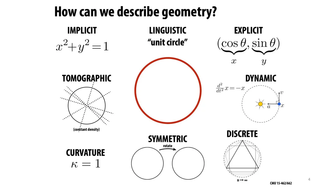
Real geometry is much harder: faces, cloth blowing in the wind, splashing water (shapes that break apart and merge again, like a fluid), a whole city with detail at different scales, a dog with long fur (a nightmare with meshes; a volumetric representation is probably better).

No one "best" choice, geometry is hard!

“I hate meshes. I cannot believe how hard this is. Geometry is hard.” (David Baraff, Senior Research Scientist, Pixar Animation Studios)

Many Ways to Digitally Encode Geometry

Slide 13

Explicit	Implicit
point cloud	level set
polygon mesh	algebraic surface
subdivision, NURBS	L-systems
…	…

Each choice is best suited to a different task or type of geometry. See Implicit and Explicit Representations.

Implicit Representations

Surfaces as an Implicit Function

Slides 14-19

Implicit representation

Points aren’t known directly, but satisfy some relationship. E.g. the unit sphere is all points with $x^2+y^2+z^2=1$. More generally:

$$f(x,y,z)=0$$

The function can be an occupancy indicator (0 outside, 1 inside, see Occupancy Field). The surface is the set of points at a threshold $\tau$ (the boundary):

$$f(\mathbf{p})=\{\begin{array}{ll}0,& \mathbf{p}\in \text{outside}\\ 1,& \mathbf{p}\in \text{inside}\end{array}\mathcal{S}=\{\mathbf{p},f(\mathbf{p})=\tau \}$$

Slide 15: a surface as the level set of an occupancy function.

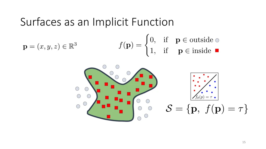
In graphics, basic primitives (ellipsoids, Gaussian blobs, …) are often combined into complex shapes. In machine learning, the implicit function has no closed form: a neural network approximates it.

A game: I'm thinking of an implicit surface $f(x,y,z)=0$. Find any point on it.

Answer Implicit surfaces make sampling hard.

Hard! You’d have to search or solve the equation.

Another game: $f(x,y,z)=x^2+y^2+z^2-1$. Is the point $(3/4,1/2,1/4)$ inside?

Answer $\frac{9}{16}+\frac{4}{16}+\frac{1}{16}=\frac{7}{8}<1$, so yes. Just plug it in. Implicit surfaces make inside/outside tests easy.

Algebraic surfaces

Slide 20

The surface is the zero set of a polynomial in $x,y,z$ (sphere, torus, heart, …). Easy to evaluate and store. But for complicated shapes (a cow, a car) it is very hard to come up with polynomials.

Constructive solid geometry

Slide 21

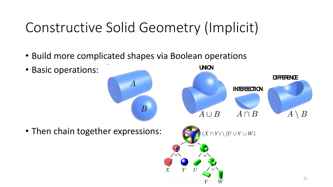
Build more complicated shapes via Boolean operations: union $A\cup B$, intersection $A\cap B$, difference $A\setminus B$. Then chain the expressions into a tree.

Slide 21: constructive solid geometry.

Blending distance functions

Slides 22-23

A distance function gives the distance to the closest point on the object. Any two distance functions $d_1,d_2$ can be blended, e.g.

$$f(x):=e^{d_1(x{)}^2}+e^{d_2(x{)}^2}-\frac{1}{2}$$

The appearance depends on how we combine them.

How do we implement a Boolean union of $d_1(x)$ and $d_2(x)$?

Answer $f(x)=\min (d_1(x),d_2(x))$.

Just take the minimum:

Whole scenes can be made of pure signed distance functions (Shadertoy). Art with math, but really hard.

Nowadays: neural distance fields

Slide 24

Storing an implicit function in a 3D grid is costly. Today, a neural network is trained to return, for every point in space, its distance to the surface. From this we recover the surface. Example: Neural Distance Fields (Chibane et al., NeurIPS 2020), which also represent open surfaces with an unsigned distance.

Slide 24: NDF, input point cloud and output.

Distance Field, Normals and Closest Points

Slide 25

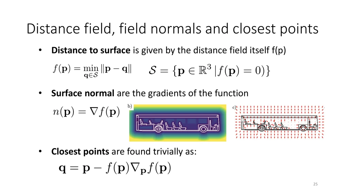
A good representation should make closest points and normals easy to compute. With a distance field this is straightforward:

Distance field

Distance to the surface is the field itself:

$$f(\mathbf{p})=\underset{\mathbf{q}\in \mathcal{S}}{\min }\Vert \mathbf{p}-\mathbf{q}\Vert \mathcal{S}=\{\mathbf{p}\in {\mathbb{R}}^3\mid f(\mathbf{p})=0\}$$

The surface normal is the gradient of the function:

$$n(\mathbf{p})=\nabla f(\mathbf{p})$$

Closest points are found trivially:

$$\mathbf{q}=\mathbf{p}-f(\mathbf{p}){\nabla }_{\mathbf{p}}f(\mathbf{p})$$

Why is the gradient the normal?

Along the level set the function does not change value. The gradient points in the direction of maximum change, so it must be orthogonal to the level set curve or surface. Hence the gradient is the normal. The closest point is found by walking the distance $f(\mathbf{p})$ against the gradient.

Slide 25: distance field and field normals.

See Signed Distance Function.

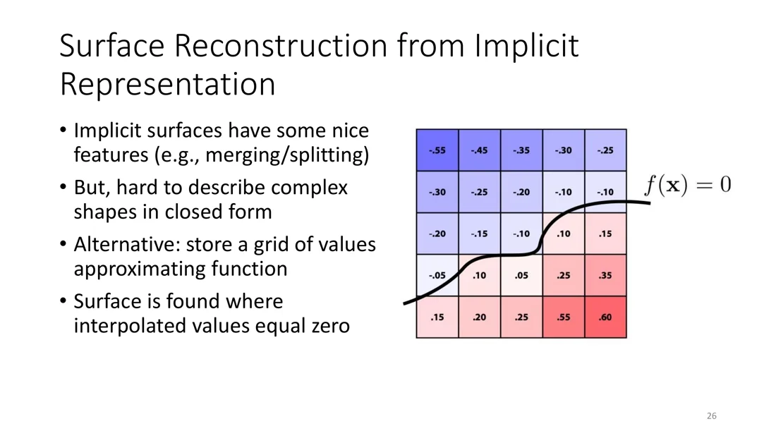
Surface Reconstruction from an Implicit Representation

Slide 26

• Implicit surfaces have nice features (e.g. merging and splitting).
• But complex shapes are hard to describe in closed form.
• Alternative: store a grid of values approximating the function.
• The surface is found where the interpolated values equal zero.

Slide 26: a grid of values, the surface is where the interpolation is zero.

Marching Cubes

Slides 27-31

Level sets are widely used in medical imaging, they are great for volumes. Marching cubes extracts a triangle mesh from them:

Marching cubes algorithm

1. Read four slices into memory.
2. Scan two slices and create a cube from four neighbors on one slice and four neighbors on the next slice.
3. Calculate an index for the cube by comparing the eight density values at the cube vertices with the surface constant (inside or outside: $2^8=256$ cases).
4. Using the index, look up the list of edges from a precalculated table.
5. Using the densities at each edge vertex, find the surface-edge intersection via linear interpolation.
6. Calculate a unit normal at each cube vertex using central differences. Interpolate the normal to each triangle vertex.
7. Output the triangle vertices and vertex normals.

Slide 27: a cube between two slices

Slide 28: the lookup table cases

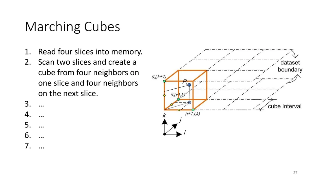
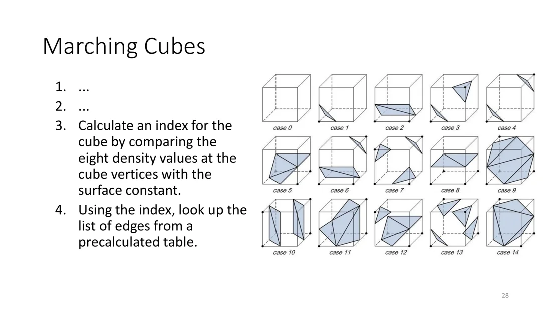
Once we have the values of the implicit function at the cube vertices, we only create mesh vertices in the cubes that the lookup table marks as crossing the surface, by interpolating along their edges.

Slide 30: the extracted contour (2D version: marching squares).

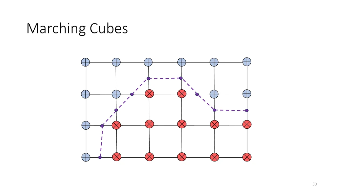
Challenges with marching cubes

• generates one polygon for each portion of the contour
• can only approximate the restriction of the contour
• fails to capture sharp details of the surface
• the generated mesh is difficult to simplify
• extracting the surface becomes challenging for higher grid sizes: a 3D uniform grid has cubic cost in the resolution

Trap

A higher resolution does not make sharp edges exact; it only costs 8 times more per doubling.

Dual Contouring

Slides 32-34

• Can capture sharp edges along the corners of a surface.
• Uses the gradient information at the edge intersections to reproduce polyhedral shapes as well as curved or sharp edges.
• Uses an octree instead of a 3D uniform grid for better efficiency.
• Uses the normals to define a Quadratic Error Function (QEF) for each leaf of the octree (inspired by Extended Marching Cubes):

Dual contouring QEF

$$E[\mathbf{x}]=\sum _i{\left({\mathbf{n}}_i\cdot (\mathbf{x}-{\mathbf{p}}_i)\right)}^2$$

${\mathbf{p}}_i,{\mathbf{n}}_i$: intersections and normals of the contour with the edges of the cube (Hermite data). One vertex $\mathbf{x}$ is placed per cell: the point that lies as well as possible on all tangent planes ($\mathbf{x}-{\mathbf{p}}_i$ must be perpendicular to the normal).

Slide 33: Hermite data, marching cubes contour and dual contour. The dual contour keeps the sharp corner.

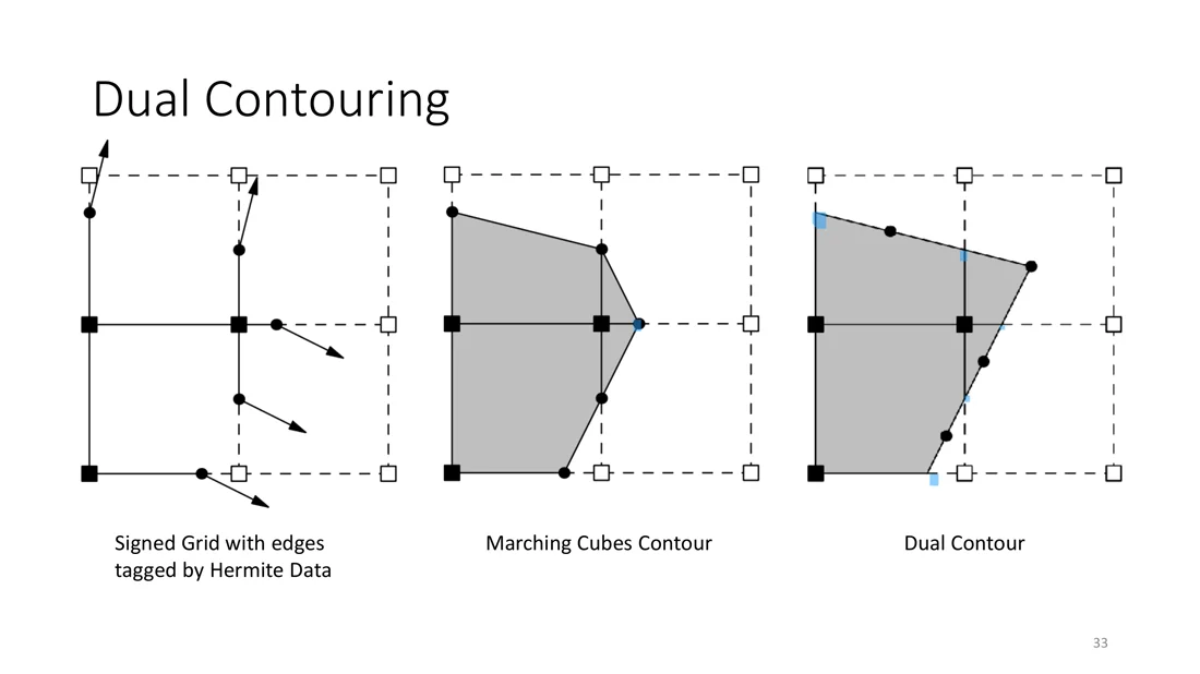
Challenges: limited expressivity because of the structured grid; very thin surfaces and features can’t be extracted faithfully (they would need a very fine grid); limited by the amount of surface simplification.

Dual Marching Cubes

Slides 35-36

• Aligns the features of the implicit function with the features of the structured grid, which enables the extraction of sharp features.
• Generates adaptive polygonalizations that are crack-free and topologically manifold.
• Reproduces thin features without excessive subdivision of the octree.

Dual marching cubes QEF

Tangent planes to $f$ at sample points $(x_i,y_i,z_i)$ over the cell $c$:

$$T_i(x,y,z)=\nabla f(x_i,y_i,z_i)\cdot \left((x,y,z)-(x_i,y_i,z_i)\right)$$ $$E(f(x,y,z),x,y,z)=\sum _i\frac{{\left(f(x,y,z)-T_i(x,y,z)\right)}^2}{1+|\nabla f(x_i,y_i,z_i){|}^2}$$

The denominator normalizes the contribution of each tangent plane.

	Dual contouring	Dual marching cubes
Samples	only on sign-changing edges of the cell	all sample points in and around the cell
Sample location	on the surface (edge crossings)	anywhere, typically cube corners
Data per sample	position + normal (Hermite data)	field value + gradient
QEF minimizes	distance to tangent planes	mismatch between local linear models and the field

Comparison and FlexiCubes

Slides 37-39

• MC fails to capture sharp features.
• DC captures sharp features, but can produce non-manifold vertices.
• DMC does not introduce non-manifold vertices and generates crack-free adaptive polygonalizations.

Slide 37: MC vs. DC vs. DMC

Slide 38: ground truth, DMC, MC, DC

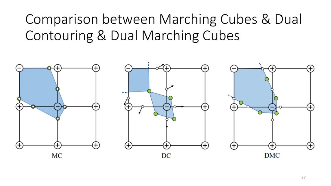
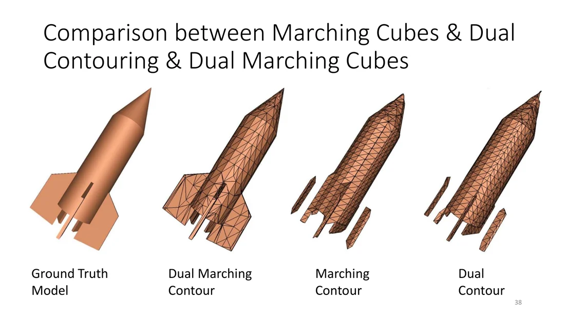
FlexiCubes (flexible iso-surface extraction): the classical methods are non-differentiable. If a neural network predicts the surface, we can’t supervise directly on the extracted mesh. FlexiCubes is an iso-surface representation designed for optimizing an unknown mesh w.r.t. geometric, visual or even physical objectives. It adds carefully chosen parameters that locally adjust the extracted mesh geometry and connectivity. They are updated together with the scalar field via automatic differentiation.

Slide 39: FlexiCubes.

Trap

FlexiCubes is not “a faster marching cubes”. Its point is that it is differentiable.

Level Sets: Storage and Pros & Cons

Slides 40-41

Although a level set gives much more explicit control over the shape (like a texture), it

• runs into problems of aliasing (unlike closed-form expressions)
• induces $O(n^3)$ storage for 3D surface extraction
• can save space by only storing a narrow band around the surface

Implicit representations: pros and cons

Pros:

• the description can be very compact (e.g. a polynomial)
• easy to determine if a point is in the shape (just plug it in!)
• other queries may also be easy (e.g. distance to the surface)
• for simple shapes, exact description, no sampling error
• easy to handle changes in topology (e.g. fluid)

Cons:

• expensive to find all points in the shape (e.g. for drawing)
• very difficult to model complex shapes

Explicit Representations

”Explicit” Representations of Geometry

Slides 42-48

Explicit representation

All points are given directly. E.g. the points on the sphere are $(\cos u\sin v,\sin u\sin v,\cos v)$ for $0\le u<2\pi$ and $0\le v\le \pi$. More generally:

$$f:{\mathbb{R}}^2\to {\mathbb{R}}^3;(u,v)\mapsto (x,y,z)$$

(There might be many of these maps, e.g. one per triangle.)

Examples: triangle meshes, polygon meshes, subdivision surfaces, NURBS, point clouds.

A game: my surface is $f(u,v)=(1.23,u,v)$. Give me some points on it.

Answer $u,v$. Explicit surfaces make sampling easy.

Just plug in any values

My surface is the torus $f(u,v)=((2+\cos u)\cos v,(2+\cos u)\sin v,\sin u)$. Is the point $(1.96,-0.39,0.9)$ inside?

Answer Explicit surfaces make inside/outside tests hard.

…No! But you can’t just plug it in.

Conclusion

Some representations work better than others, it depends on the task!

	Implicit	Explicit
Inside/outside test	easy (plug in)	hard
Sampling points	hard	easy (plug in $u,v$)

Point Clouds

Slide 49

• Easiest representation: a list of points $(x,y,z)$, often augmented with normals.
• Easily represents any kind of geometry.
• Easy to draw a dense cloud ($\gg 1$ point per pixel).
• Hard to interpolate under-sampled regions.
• Hard to do processing, simulation, …

Point clouds are the output of many 3D scanners and reconstruction methods (SfM, MVS). See Point Cloud.

From Points to Surfaces: Poisson Surface Reconstruction

Slides 50-54

Why do we need surface reconstruction?

• Point clouds are discrete and unordered: no connectivity or topology.
• Downstream tasks (rendering, simulation, 3D printing) need a continuous surface.
• Goal: a method that is global, robust to noise, and produces watertight meshes.
• Key idea: recast surface reconstruction as solving a Poisson equation.

Reconstructing a surface from a point cloud is underdetermined. Given an oriented point cloud, we look for an indicator function ${\chi }_M$ (1 inside, 0 outside). Its gradient is zero almost everywhere (the indicator is constant almost everywhere), except near the surface, where it equals the inward surface normal. So the oriented point samples can be viewed as samples of the gradient of the indicator function.

Slide 51: oriented points V → indicator gradient ∇χ → indicator function χ → surface ∂M (Kazhdan et al., 2006).

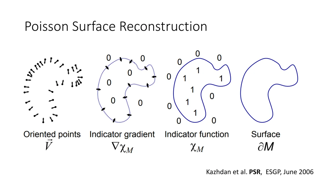
Poisson surface reconstruction (Kazhdan et al., 2006)

Given an oriented point cloud with points $p_1,\dots ,p_n$ and outward normals $n_1,\dots ,n_n$, find $f:{\mathbb{R}}^d\to \mathbb{R}$ with

$$f(p_i)=0,\nabla f(p_i)=n_i,\forall i\in \{1,\dots ,n\}$$

Step 1: interpolate the normals into a vector field with a convolutional kernel $F$, in a box $B$ containing the points:

$$V(x)=\sum _{i}F(x,x_i)n_i$$

Step 2: find the function whose gradient best matches $V$:

$$f=\arg \underset{g}{\min }{\int }_B\Vert V(x)-\nabla g(x){\Vert }_2^{2}dx$$

This variational problem is equivalent to the Poisson equation

$$\Delta f=\nabla \cdot V(x)$$

solved by discretization with the finite element method on an octree and a purpose-built multigrid algorithm.

Screened PSR (Kazhdan and Hoppe, 2013) adds a term that pulls the function to zero at the input points:

$$f=\arg \underset{g}{\min }{\int }_B\Vert V(x)-\nabla g(x){\Vert }_2^{2}dx+\alpha \sum _{i}g(p_i{)}^2$$

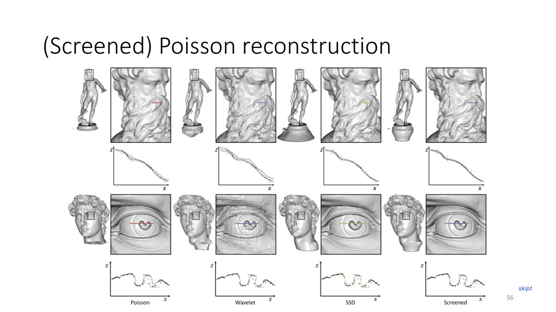
(Screened) Poisson Reconstruction

Slides 55-60

• It can extract the surface from oriented point clouds.
• Screened PSR efficiently implements sparsity constraints and captures the details of the surface better.
• Screened PSR uses an efficient octree and multigrid algorithm to reduce the time complexity.

However, these methods only output the likeliest surface given the points and their assumed prior. In reality there could be infinitely many surfaces for the same set of points with normals.

In the comparison, Poisson reconstruction (and to a lesser extent SSD) over-smooths the data, wavelet reconstruction has derivative discontinuities, and screened Poisson fits the samples faithfully without introducing noise.

Slide 56: Poisson, wavelet, SSD and screened Poisson reconstructions.

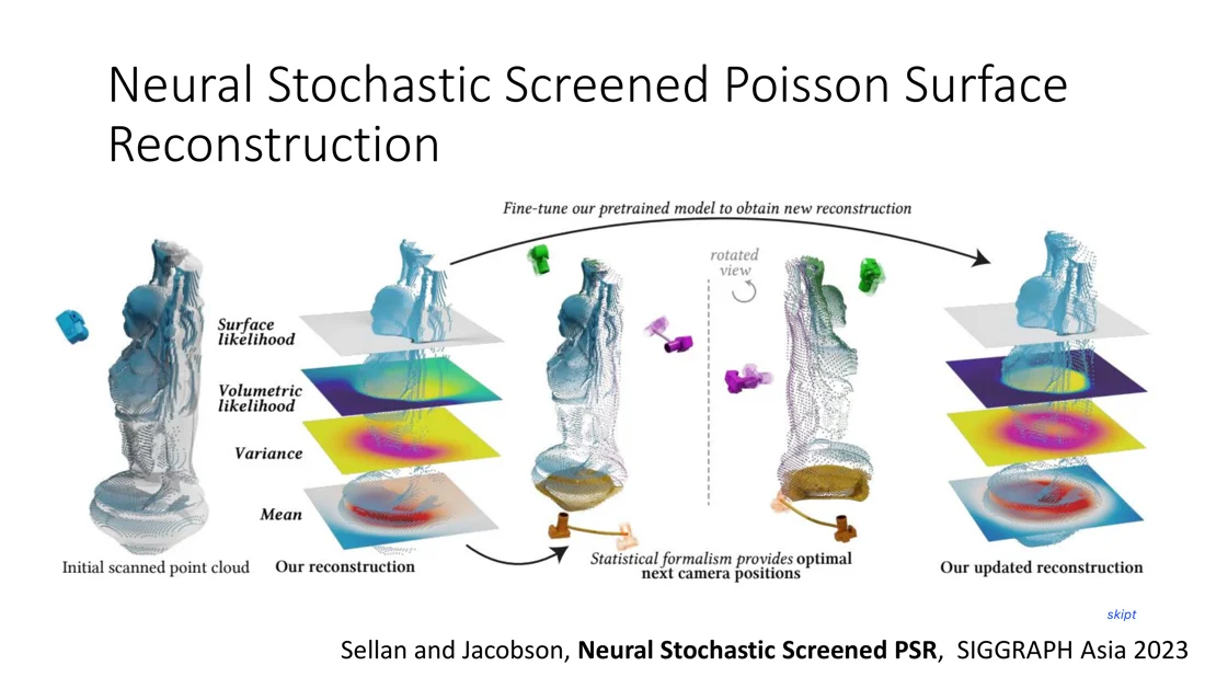
Neural Stochastic Screened PSR (Sellan and Jacobson, SIGGRAPH Asia 2023) goes a step further: it models the posterior distribution (a Gaussian) over all possible reconstructions. Mean and covariance of the implicit field are parameterized with neural networks and optimized with gradient-based methods on losses derived from the variational Poisson equation. This allows statistical queries: the probability that a point is inside the shape, $P(x\in \Omega )$, or on the surface. In theory it strictly generalizes PSR; in practice its volumetric smoothness prior avoids overfitting. It can even suggest where to scan next.

Slide 58: neural stochastic screened PSR.

Trap

PSR does not interpolate the points exactly, it smooths (over-smoothing). Screened PSR still needs normals: the gradient term remains.

Polygon Meshes

Slides 61-64

• Store vertices and polygons (most often triangles or quads).
• Easier processing and simulation, adaptive sampling.
• More complicated data structures, irregular neighborhoods.
• Lightweight and easy to manipulate. Problem: topology!

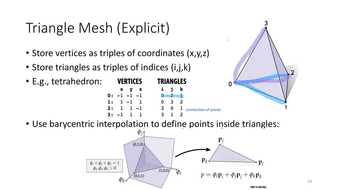
Triangle mesh:

• vertices as triples of coordinates $(x,y,z)$
• triangles as triples of vertex indices $(i,j,k)$ (e.g. a tetrahedron: 4 vertices, 4 triangles)
• points inside a triangle via barycentric interpolation: $p={\varphi }_i{p}_i+{\varphi }_j{p}_j+{\varphi }_k{p}_k$ with ${\varphi }_i+{\varphi }_j+{\varphi }_k=1$, $\varphi \ge 0$

Slide 62: triangle mesh and barycentric interpolation.

Mesh normals

Option 1, one normal per face:

$$n=(p_2-p_1)\times (p_3-p_1)$$

Option 2, interpolate the incident face normals at each vertex, then use barycentric interpolation inside the triangle:

$$n({\varphi }_1,{\varphi }_2,{\varphi }_3)={\varphi }_1{n}_1+{\varphi }_2{n}_2+{\varphi }_3{n}_3$$

Distance queries and closest points:

• Smooth parametric surface: evaluation $f(u,v)$, normals $n(u,v)=f_u(u,v)\times f_v(u,v)$. The closest surface point to $\mathbf{q}$ is the $f(u,v)$ with $[\mathbf{q}-f(u,v)]\times \mathbf{n}(u,v)=0$ (the difference is parallel to the normal).
• Mesh: find the closest triangle, then the closest point in that triangle. Use a kd-tree or AABB tree to find the closest triangles.

See Mesh.

Subdivision

Slides 65-68

An alternative starting point for curves and surfaces:

• Start with a “control curve”.
• Repeatedly split, and take a weighted average to get new positions.
• For a careful choice of averaging rule, this approaches a nice limit curve, often exactly the same curve as well-known spline schemes!

Slide 65: subdivision of a control curve.

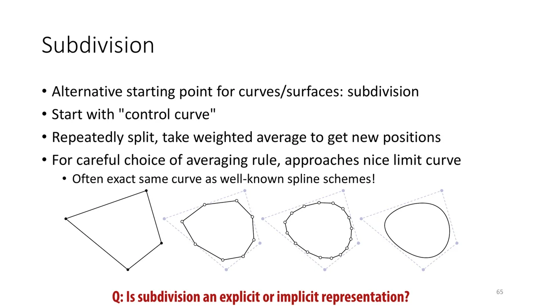
Is subdivision an explicit or an implicit representation?

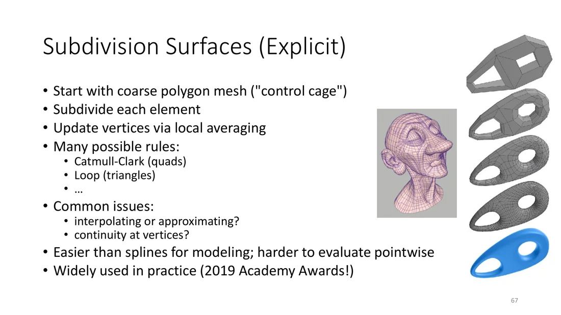
Answer Explicit (Slide 67). There is no level set; the points are generated directly from the control cage (even though we don't know them in closed form before subdividing).

Subdivision surfaces:

• Start with a coarse polygon mesh (“control cage”), subdivide each element, update the vertices via local averaging.
• Many possible rules: Catmull-Clark (quads), Loop (triangles), …
• Common issues: interpolating or approximating (does the limit surface pass through the control points?), continuity at vertices (where more or fewer than 4 patches meet).
• Easier than splines for modeling; harder to evaluate pointwise.
• Widely used in practice: one of the first uses in animation was Pixar’s short film Geri’s Game. Tony DeRose, Michael Kass and Tien Truong received an Academy Award for their work on subdivision surfaces. In computer vision, e.g. What shapes are dolphins? (Cashman & Fitzgibbon).

Slide 67: subdivision surfaces.

Part 2: Procrustes Alignment

Aligning Point Clouds to a Common Frame

Slides 70-72, 86-99

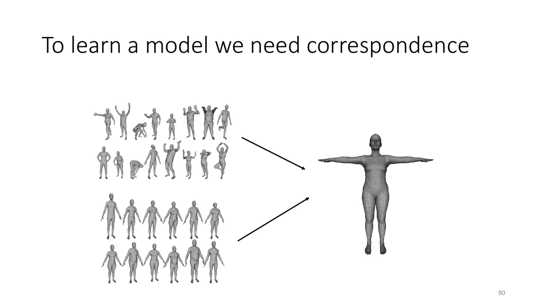
Motivation: to learn a model of human pose and shape (like SMPL, $M({\mathbf{X}}_{pose},{\mathbf{X}}_{shape})$), we scan a lot of people in lots of poses. To learn a model we need correspondences between all these scans and a template. That needs non-rigid articulated registration; the first step is rigid alignment.

Slide 90: to learn a model we need correspondence.

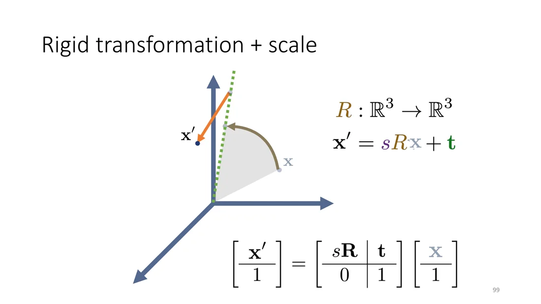
A mesh is $\mathcal{V}\equiv \{\mathbf{F}\in {\mathbb{N}}^{M\times 3},\mathbf{X}\in {\mathbb{R}}^{N\times 3}\}$ (faces and vertices). How can we transform the set of points $\mathbf{X}$?

$$\text{translate: }{\mathbf{X}}^{\prime }=\mathbf{X}+\mathbf{t},\mathbf{t}\in {\mathbb{R}}^3\text{rotate: }{\mathbf{X}}^{\prime T}=\mathbf{R}{\mathbf{X}}^T,\mathbf{R}\in SO(3)\text{scale: }{\mathbf{X}}^{\prime }=s\mathbf{X},s\in \mathbb{R}$$

Combined: ${\mathbf{x}}^{\prime }=s\mathbf{Rx}+\mathbf{t}$, or in homogeneous coordinates

$$\left[\begin{array}{c}{\mathbf{x}}^{\prime }\\ 1\end{array}\right]=\left[\begin{array}{cc}s\mathbf{R}& \mathbf{t}\\ 0& 1\end{array}\right]\left[\begin{array}{c}\mathbf{x}\\ 1\end{array}\right]$$

Slide 99: rigid transformation + scale.

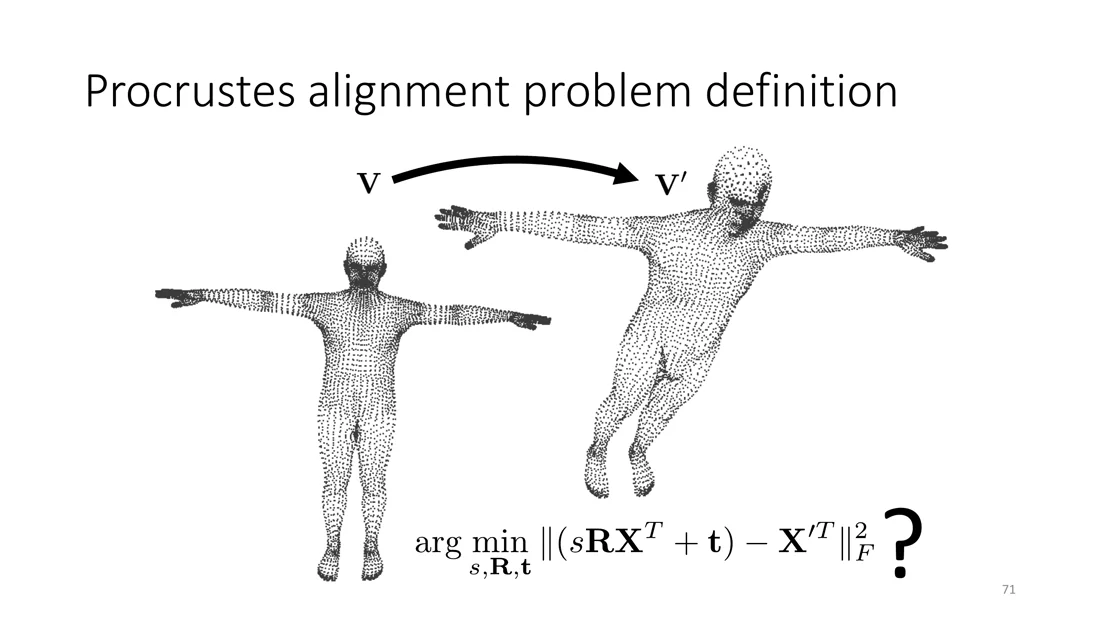
Procrustes alignment problem

Given two point sets $\mathbf{V}$ and ${\mathbf{V}}^{\prime }$ with known correspondences, find scale, rotation and translation:

$$\arg \underset{s,\mathbf{R},\mathbf{t}}{\min }{\Vert (s\mathbf{R}{\mathbf{V}}^T+\mathbf{t})-{\mathbf{V}}^{\prime T}\Vert }_F^2$$

Name: Procrustes is a bandit from Greek mythology who made his victims fit his bed by stretching their limbs or cutting them off (“he who stretches”).

Slide 71: the Procrustes alignment problem.

Optimization Problem and SVD Recap

Slides 73-74

$$s,\mathbf{R},\mathbf{t}=\arg \underset{s,\mathbf{R},\mathbf{t}}{\min }\sum _i\Vert s\mathbf{R}{\mathbf{x}}_i+\mathbf{t}-{\mathbf{y}}_i{\Vert }^2$$

Is it linear or quadratic in the parameters? Quadratic in $\mathbf{t}$ and $s$, but $\mathbf{R}$ must stay a rotation. It still has a closed-form solution, with the SVD:

$$\mathbf{A}=\mathbf{U}\Sigma {\mathbf{V}}^T,\mathbf{A}\in {\mathbb{R}}^{M\times N}\text{ real},\mathbf{U}(M\times M)\text{ and }\mathbf{V}(N\times N)\text{ orthogonal},\Sigma (M\times N)\text{ diagonal}$$

Warning

The $\mathbf{V}$ of the SVD is not the vertex matrix!

Procrustes Solution

Slide 75

Procrustes alignment steps

Matrices of points $\mathbf{X}=[{\mathbf{x}}_1\dots {\mathbf{x}}_n{]}^T$, $\mathbf{Y}=[{\mathbf{y}}_1\dots {\mathbf{y}}_n{]}^T\in {\mathbb{R}}^{N\times 3}$, centered versions $\bar{\mathbf{X}},\bar{\mathbf{Y}}$ (centroid subtracted).

Rotation: SVD of the point cross-covariance

$${\bar{\mathbf{Y}}}^T\bar{\mathbf{X}}=\mathbf{U}\Sigma {\mathbf{V}}^T,\mathbf{R}=\mathbf{U}{\mathbf{V}}^T$$

Scale: a quotient of eigenvalue sums

$$s=\frac{\text{tr}(\Sigma )}{\Vert \bar{\mathbf{X}}{\Vert }_F^2}$$

Translation: the centroid difference

$$\mathbf{t}=\bar{\mathbf{y}}-s\mathbf{R}\bar{\mathbf{x}}$$

($\bar{\mathbf{x}},\bar{\mathbf{y}}$ here are the centroids.)

Sign of t

Slide 75 writes $\mathbf{t}=s\mathbf{R}\bar{\mathbf{x}}-\bar{\mathbf{y}}$, but the derivation on Slide 78 gives $\mathbf{t}=\bar{\mathbf{y}}-s\mathbf{R}\bar{\mathbf{x}}$. The derivation is right: with $\mathbf{y}=s\mathbf{Rx}+\mathbf{t}$, the centroids must map onto each other.

Trap

Procrustes does not find correspondences. They are its input.

Proof

Slides 76-84

Derivation: translation (Slides 77-78)

$$E\equiv \sum _i\Vert s\mathbf{R}{\mathbf{x}}_i+\mathbf{t}-{\mathbf{y}}_i{\Vert }^2=\sum _i{s}^2{\mathbf{x}}_i^T{\mathbf{x}}_i+{\mathbf{t}}^T\mathbf{t}+{\mathbf{y}}_i^T{\mathbf{y}}_i+2s{\mathbf{x}}_i^T{\mathbf{R}}^T\mathbf{t}-2s{\mathbf{x}}_i^T{\mathbf{R}}^T{\mathbf{y}}_i-2{\mathbf{t}}^T{\mathbf{y}}_i$$

Remove the terms that don’t depend on $\mathbf{t}$. With the centroids $\bar{\mathbf{x}}=\frac{{\sum }_i{\mathbf{x}}_i}{N}$, $\bar{\mathbf{y}}=\frac{{\sum }_i{\mathbf{y}}_i}{N}$:

$$\mathbf{t}=\arg \underset{\mathbf{t}}{\min }{\mathbf{t}}^T(2s\mathbf{R}\bar{\mathbf{x}}+\mathbf{t}-2\bar{\mathbf{y}})=\bar{\mathbf{y}}-s\mathbf{R}\bar{\mathbf{x}}$$

So given $s$ and $\mathbf{R}$, we can compute the translation.

Derivation: rotation (Slides 79-83)

Subtract the centroids (${\bar{\mathbf{x}}}_i\equiv {\mathbf{x}}_i-\bar{\mathbf{x}}$, ${\bar{\mathbf{y}}}_i\equiv {\mathbf{y}}_i-\bar{\mathbf{y}}$) to get a simpler expression, subject to $\mathbf{R}\in SO(3)$:

$$E=\sum _i\Vert s\mathbf{R}{\mathbf{x}}_i+\mathbf{t}-{\mathbf{y}}_i{\Vert }^2=\sum _i\Vert s\mathbf{R}{\bar{\mathbf{x}}}_i-{\bar{\mathbf{y}}}_i{\Vert }^2$$

The optimal rotation does not depend on the scale:

$$\begin{array}{rl}\mathbf{R}& =\arg \underset{\mathbf{R}}{\min }\Vert \mathbf{R}{\bar{\mathbf{X}}}^T-{\bar{\mathbf{Y}}}^T{\Vert }_F^2\\ & =\arg \underset{\mathbf{R}}{\min }\Vert \mathbf{R}{\bar{\mathbf{X}}}^T{\Vert }_F^2+\Vert {\bar{\mathbf{Y}}}^T{\Vert }_F^2-2⟨\mathbf{R}{\bar{\mathbf{X}}}^T,{\bar{\mathbf{Y}}}^T{⟩}_F\\ & =\arg \underset{\mathbf{R}}{\min }\Vert {\bar{\mathbf{X}}}^T{\Vert }_F^2+\Vert {\bar{\mathbf{Y}}}^T{\Vert }_F^2-2⟨\mathbf{R}{\bar{\mathbf{X}}}^T,{\bar{\mathbf{Y}}}^T{⟩}_F\text{(rotation does not change the norm)}\\ & =\arg \underset{\mathbf{R}}{\max }⟨\mathbf{R},{\bar{\mathbf{Y}}}^T\bar{\mathbf{X}}{⟩}_F\text{(inner product should be maximal; cross-covariance)}\\ & =\arg \underset{\mathbf{R}}{\max }⟨\mathbf{R},\mathbf{U}\Sigma {\mathbf{V}}^T{⟩}_F\text{(SVD)}\\ & =\arg \underset{\mathbf{R}}{\max }⟨{\mathbf{U}}^T\mathbf{RV},\Sigma {⟩}_F=\arg \underset{\mathbf{R}}{\max }⟨S,\Sigma {⟩}_F,S={\mathbf{U}}^T\mathbf{RV}\end{array}$$

What kind of matrix is $S$? Orthogonal. What kind is $\Sigma$? Diagonal (non-negative). So the inner product is maximal when $S$ equals the identity:

$$I={\mathbf{U}}^T\mathbf{RV}⟹\mathbf{R}=\mathbf{U}{\mathbf{V}}^T$$

Derivation: scale (Slide 84)

Optimize the scale given the rotation:

$$s=\arg \underset{s}{\min }\left(s^2\sum _i{\bar{\mathbf{x}}}_i^T{\bar{\mathbf{x}}}_i-2s\sum _i{\bar{\mathbf{x}}}_i^T{\mathbf{R}}^T{\bar{\mathbf{y}}}_i\right)=\arg \underset{s}{\min }(s^{2}a-2sb)=\frac{b}{a}=\frac{{\sum }_i{\bar{\mathbf{x}}}_i^T{\mathbf{R}}^T{\bar{\mathbf{y}}}_i}{{\sum }_i{\bar{\mathbf{x}}}_i^T{\bar{\mathbf{x}}}_i}$$ $$=\frac{\text{tr}(\bar{\mathbf{X}}{\mathbf{R}}^T{\bar{\mathbf{Y}}}^T)}{\Vert \bar{\mathbf{X}}{\Vert }_F^2}=\frac{\text{tr}({\mathbf{R}}^T{\bar{\mathbf{Y}}}^T\bar{\mathbf{X}})}{\Vert \bar{\mathbf{X}}{\Vert }_F^2}=\frac{\text{tr}(\mathbf{V}{\mathbf{U}}^T\mathbf{U}\Sigma {\mathbf{V}}^T)}{\Vert \bar{\mathbf{X}}{\Vert }_F^2}=\frac{\text{tr}(\Sigma )}{\Vert \bar{\mathbf{X}}{\Vert }_F^2}$$

Used: 1) the trace is invariant to cyclic shifts, 2) ${\bar{\mathbf{Y}}}^T\bar{\mathbf{X}}=\mathbf{U}\Sigma {\mathbf{V}}^T$, $\mathbf{R}=\mathbf{U}{\mathbf{V}}^T$, 3) the trace equals the sum of eigenvalues for square matrices.

Note

In practice one also checks $\det (\mathbf{U}{\mathbf{V}}^T)$: if it is $-1$, the result is a reflection, and the sign of the last column of $\mathbf{U}$ is flipped. This is not on the slides.

Part 3: Iterative Closest Point (ICP)

What Is Missing?

Slides 117-126

Given correspondences, Procrustes finds the optimal rigid alignment. Problems:

• How do we find the correspondences between shapes?
• How do we align shapes non-rigidly?

Two tools: ICP optimizes alignment and correspondences together; continuous optimization handles general deformations.

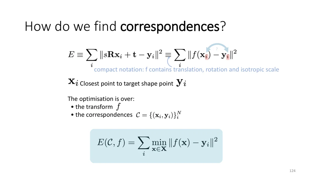
The optimization is over the transform $f$ and the correspondences $\mathcal{C}=\{({\mathbf{x}}_i,{\mathbf{y}}_i){\}}_i^N$. With ${\mathbf{x}}_i$ the closest point to the target shape point ${\mathbf{y}}_i$ (and $f$ containing translation, rotation and isotropic scale):

$$E\equiv \sum _i\Vert s\mathbf{R}{\mathbf{x}}_i+\mathbf{t}-{\mathbf{y}}_i{\Vert }^2\equiv \sum _i\Vert f({\mathbf{x}}_i)-{\mathbf{y}}_i{\Vert }^{2}E(\mathcal{C},f)=\sum _i\underset{\mathbf{x}\in \mathbf{X}}{\min }\Vert f(\mathbf{x})-{\mathbf{y}}_i{\Vert }^2$$

Slide 124: optimize over the transform and the correspondences.

Solution: Iteratively Find Correspondences

Slides 127-138

What if we estimate the correspondences? Alternate between the two:

Alternation

Given the current best transformation, which are the closest correspondences?

$${\mathbf{x}}_i^{j+1}=\arg \underset{\mathbf{x}\in \mathbf{X}}{\min }\Vert f^j(\mathbf{x})-{\mathbf{y}}_i{\Vert }^2$$

Given the current best correspondences, which is the best transformation? (solved with Procrustes)

$$f^{j+1}=\arg \underset{f}{\min }\sum _i\Vert f({\mathbf{x}}_i^{j+1})-{\mathbf{y}}_i{\Vert }^2$$

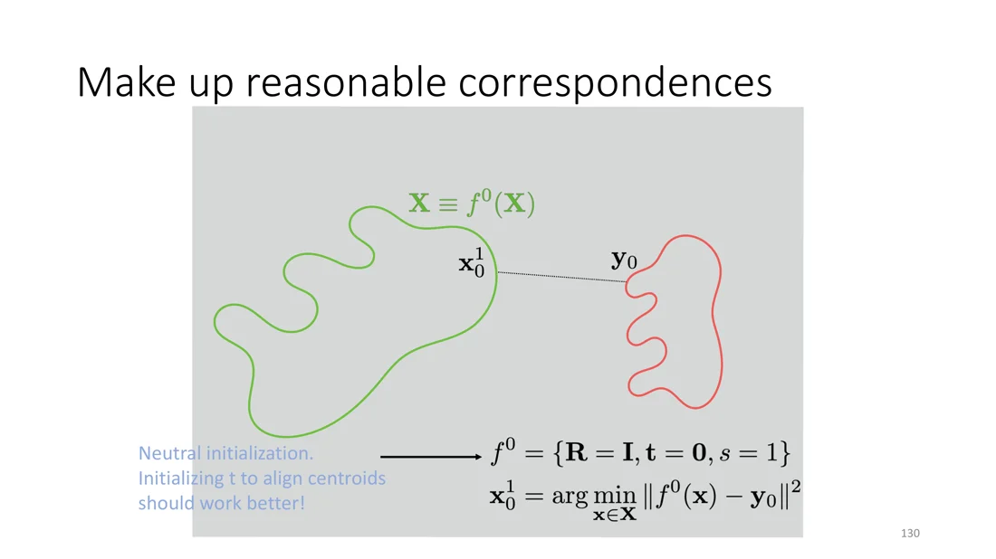
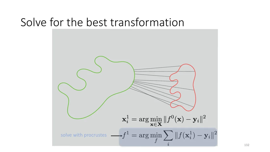
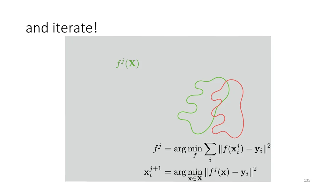
Walkthrough on the slides: start with a neutral initialization $f^0=\{\mathbf{R}=\mathbf{I},\mathbf{t}=0,s=1\}$ (initializing $\mathbf{t}$ to align the centroids should work better!), make up reasonable correspondences (closest points), solve for the best transformation with Procrustes, apply it, and iterate until the shapes overlap.

Slide 130: closest points

Slide 132: solve with Procrustes

Slide 135: iterate

The ICP Algorithm

Slides 139-143

Iterative Closest Point (ICP)

1. Initialize (typically better than 0: align the centroids)

$$f^0=\left\{\mathbf{R}=\mathbf{I},\mathbf{t}=\frac{\sum {\mathbf{y}}_i}{N}-\frac{\sum {\mathbf{x}}_i}{N},s=1\right\}$$

2. Compute correspondences according to the current best transform:

$${\mathbf{x}}_i^{j+1}=\arg \underset{\mathbf{x}\in \mathbf{X}}{\min }\Vert f^j(\mathbf{x})-{\mathbf{y}}_i{\Vert }^2$$

3. Compute the optimal transformation $(s,\mathbf{R},\mathbf{t})$ with Procrustes:

$$f^{j+1}=\arg \underset{f}{\min }\sum _i\Vert f({\mathbf{x}}_i^{j+1})-{\mathbf{y}}_i{\Vert }^2$$

4. Terminate if converged (error below a threshold), otherwise iterate.
5. Converges to local minima.

flowchart LR
  I["Initialize f⁰<br/>(align centroids)"] --> C["Closest points<br/>(correspondences)"]
  C --> P["Procrustes:<br/>best s, R, t"]
  P --> A["Apply transform"]
  A --> T{"Converged?"}
  T -- "no" --> C
  T -- "yes" --> D["Done<br/>(local minimum)"]

Trap

ICP finds only a local minimum, not the global optimum. A bad initialization gives a wrong alignment.

Is ICP the Best We Can Do?

Slides 144-150

Computing closest points:

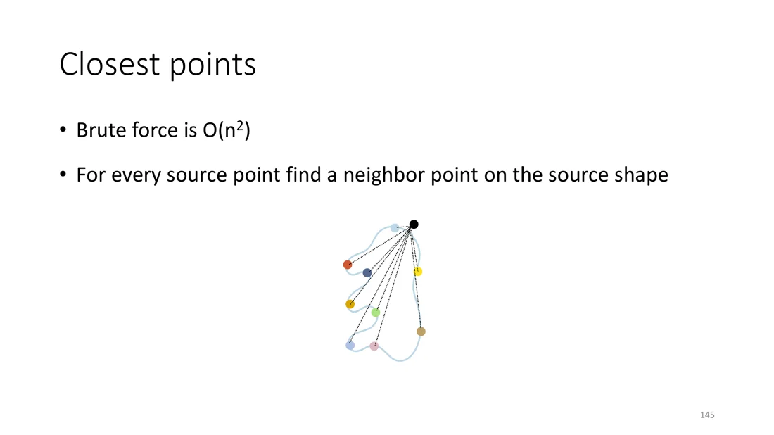
• Brute force is $O(n^2)$ (for every point, check every point).
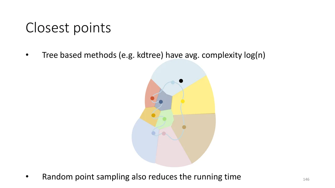
• Tree-based methods (e.g. kd-tree) have an average complexity of $\log (n)$ per query.
• Random point sampling also reduces the running time.

Slide 145: brute force O(n²)

Slide 146: kd-tree

ICP: tips to avoid local minima

• Always find correspondences from target to source (proper data term).
• Outliers → robust cost functions.
• Use additional information (e.g. normals).
• Compute the transformation from greedy subsets of points: RANSAC.

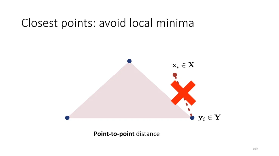
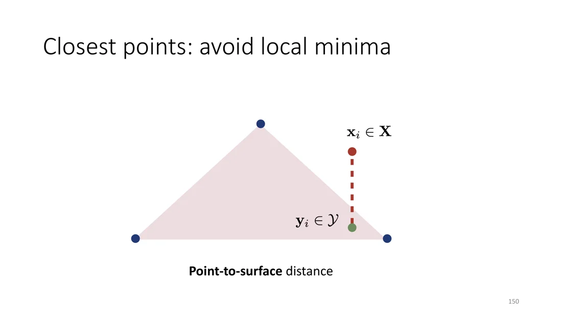
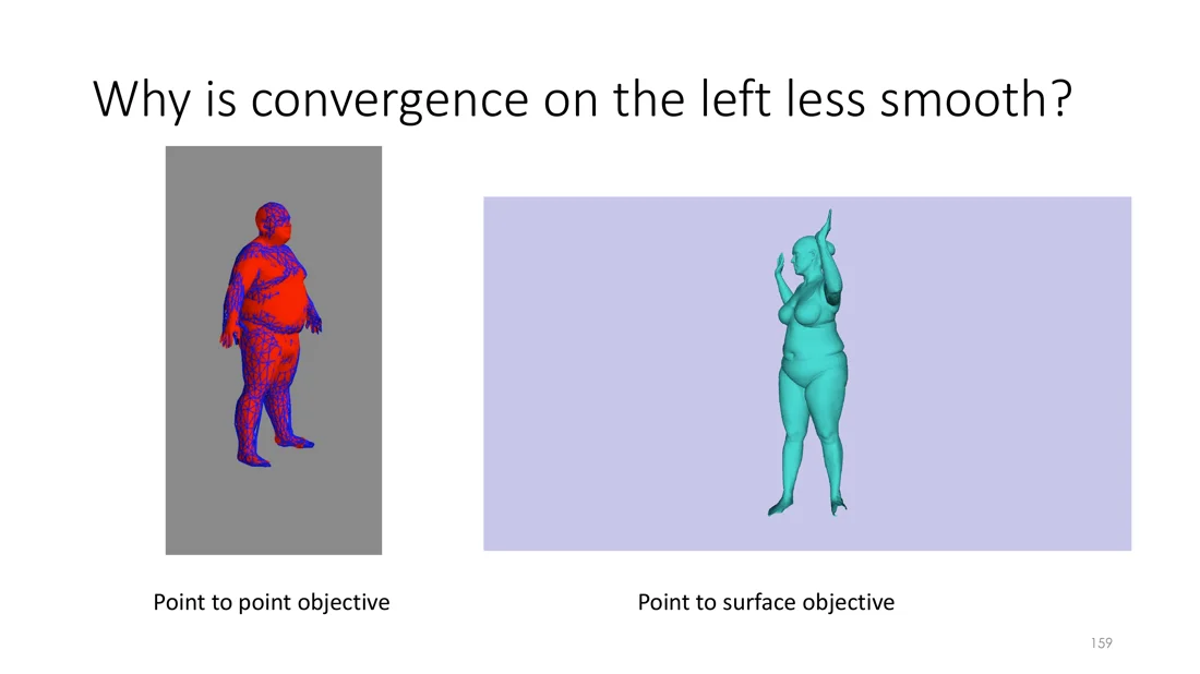
A much better objective: point-to-surface distance. Instead of the distance to the closest vertex of the target mesh (point-to-point), use the distance to the closest point on the surface (point-to-surface). The point-to-point closest vertex can be far away from the real closest surface point.

Slide 149: point-to-point

Slide 150: point-to-surface

Gradient-Based ICP

Slides 151-166

Procrustes gives the optimal rigid transformation and scale for given correspondences. What if the deformation model is not rigid? Can we generalize ICP to non-rigid deformation?

Instead of the optimal transformation, we only compute a transform that reduces the error: a descent step, by linearizing the energy (the Jacobian of the distance-based energy).

$$\arg \underset{f}{\min }E(f)=\arg \underset{f}{\min }\sum _i\Vert f({\mathbf{x}}_i^{j+1})-{\mathbf{y}}_i{\Vert }^2$$

• If $f$ is a rigid transformation, we can solve this with Procrustes.
• If $f$ is a general non-linear function: gradient descent $f^{k+1}=f^k-\lambda {\nabla }_{f}E(f)$.
• For least squares there is a better method: Gauss-Newton based methods.

Gradient-based ICP

1. Energy: $E\equiv {\sum }_i\Vert {\min }_{\mathbf{x}}f(\mathbf{x})-{\mathbf{y}}_i{\Vert }^2$
2. Consider the correspondences fixed in each iteration $j+1$: ${\mathbf{x}}_i^{j+1}=\arg {\min }_{\mathbf{x}\in \mathbf{X}}\Vert f^j(\mathbf{x})-{\mathbf{y}}_i{\Vert }^2$
3. Compute the gradient of the energy around the current estimate: $g^{j+1}=\nabla E(f^j)$
4. Apply a step (gradient descent, dogleg, LM, BFGS, …): $f^{j+1}=k_{step}(g^{0\dots j+1},f^{0\dots j})$, for example $f^{j+1}=f^j-\alpha g^{j+1}$
5. Terminate if converged, otherwise iterate (go to step 2).

Slide 159: why is convergence with the point-to-point objective (left) less smooth? The correspondences jump between vertices.

The gradient is the derivative of the sum of squared distances w.r.t. the parameters of $f$. Each derivative is easy, but nobody wants to write them all down: chain rule and automatic differentiation. Write the energy as if it was numpy code; it becomes an expression tree with Jacobians available at each step.

Why gradient-based ICP?

• The formulation is much more generic: the energy can include other terms, more parameters, etc.
• Lots of software for solving the least squares problem (cvx, Ceres, …).
• However, for general deformation models the energy is non-convex. The optimization can get trapped in local minima.

Take-home message

• Procrustes is optimal for rigid alignment problems with known correspondences.
• For other problems, compute correspondences and solve for the best transformation iteratively with ICP.

Putting It Together: From a Point Cloud to a Mesh

The exam scenario: a museum has a point cloud of a statue (200 points) and wants a mesh, using a signed distance field. This page covers the classical tools; the learned SDF (DeepSDF, neural implicits) follows in Lecture 6.1.

flowchart LR
  P["Point cloud<br/>(+ normals)"] --> F["Implicit field<br/>SDF / indicator<br/>(PSR, or a network)"]
  F --> G["Evaluate on a grid"]
  G --> M["Marching cubes<br/>(level set f = 0)"]
  M --> O["Triangle mesh"]

Step	What it needs	Notes
Point cloud → implicit field	oriented normals for PSR; for a learned SDF, a trained network	inside/outside comes from the normals (PSR) or is learned
Field → grid	evaluate $f$ at grid vertices	cubic cost in the resolution
Grid → mesh	marching cubes on the zero level set	sharp features lost; dual contouring / DMC are better; FlexiCubes if it has to be differentiable

Training vs. inference (for a learned SDF)

Training: a network learns to predict the signed distance (or occupancy) of 3D query points from data where the ground truth distances are known (needs watertight shapes). Inference: encode the new point cloud, query the network on a dense grid, run marching cubes on the zero level set to get the mesh.

Why can't we compute a signed distance directly from the raw point cloud?

Answer sign needs inside and outside, which a raw, unordered point cloud does not define (no connectivity, possibly holes). PSR gets inside/outside from the normals; a learned method gets it from training data with watertight ground truth. An unsigned distance (like NDF) does not need it.

The

Self-Test

What is the difference between implicit and explicit representations? Which tasks does each make easy?

Answer $f(x,y,z)=0$; inside/outside tests are easy (plug in), sampling is hard. Explicit: points are given directly, $f(u,v)\mapsto (x,y,z)$; sampling is easy, inside/outside tests are hard.

Implicit: points satisfy a relationship

How do you get the normal and the closest surface point from a distance field?

Answer $n(\mathbf{p})=\nabla f(\mathbf{p})$ (the gradient is orthogonal to the level set). Closest point $\mathbf{q}=\mathbf{p}-f(\mathbf{p})\nabla f(\mathbf{p})$.

Normal

How do you implement the union of two distance functions?

Answer $f(x)=\min (d_1(x),d_2(x))$.

Describe marching cubes and its weaknesses.

Answer

Build cubes from two slices, compute an 8-bit index from the inside/outside signs of the corners, look up the edge list in a precalculated table, place vertices on the edges by linear interpolation, compute normals by central differences, output triangles. Weaknesses: misses sharp features, only approximates the contour, hard to simplify, cubic cost in the resolution.

What does dual contouring do better, and what does it need?

Answer ${\sum }_i({\mathbf{n}}_i\cdot (\mathbf{x}-{\mathbf{p}}_i){)}^2$. It needs Hermite data (edge intersections + normals) and uses an octree. It can produce non-manifold vertices; DMC avoids that.

It captures sharp edges and corners by placing one vertex per cell that minimizes the QEF

Why FlexiCubes?

Answer

Classical extraction is non-differentiable, so a network can’t be supervised on the extracted mesh. FlexiCubes adds parameters that are optimized with the field via automatic differentiation.

Explain Poisson surface reconstruction.

Answer $V$, find $f$ whose gradient best matches $V$ (${\min }_g\int \Vert V-\nabla g{\Vert }^2$), which is the Poisson equation $\Delta f=\nabla \cdot V$, solved on an octree with multigrid. Extract the surface (e.g. marching cubes). Screened PSR adds $\alpha {\sum }_{i}g(p_i{)}^2$.

Oriented points are samples of the gradient of the indicator function. Interpolate the normals into a vector field

Is subdivision explicit or implicit?

Answer

Explicit.

Give the Procrustes solution for $s$, $\mathbf{R}$, $\mathbf{t}$.

Answer ${\bar{\mathbf{Y}}}^T\bar{\mathbf{X}}=\mathbf{U}\Sigma {\mathbf{V}}^T$, $\mathbf{R}=\mathbf{U}{\mathbf{V}}^T$, $s=\frac{\text{tr}(\Sigma )}{\Vert \bar{\mathbf{X}}{\Vert }_F^2}$, $\mathbf{t}=\bar{\mathbf{y}}-s\mathbf{R}\bar{\mathbf{x}}$ (centroids).

With centered point matrices:

Why is $\mathbf{R}=\mathbf{U}{\mathbf{V}}^T$ optimal?

Answer $\Vert \mathbf{R}{\bar{\mathbf{X}}}^T-{\bar{\mathbf{Y}}}^T{\Vert }_F^2$ equals maximizing $⟨\mathbf{R},\mathbf{U}\Sigma {\mathbf{V}}^T{⟩}_F=⟨{\mathbf{U}}^T\mathbf{RV},\Sigma {⟩}_F$. $S={\mathbf{U}}^T\mathbf{RV}$ is orthogonal and $\Sigma$ diagonal with non-negative entries, so the maximum is at $S=I$.

Minimizing

Describe ICP. What does it converge to?

Answer

Initialize (align centroids), then alternate: closest-point correspondences for the current transform, optimal transform with Procrustes, apply, until the error is below a threshold. It converges to a local minimum.

How can ICP be improved?

Answer $\log n$), correspondences from target to source, robust cost functions against outliers, normals, RANSAC, point-to-surface instead of point-to-point distances, and gradient-based ICP (Gauss-Newton, autodiff) for non-rigid deformation models.

kd-trees for closest points (

Related

• Previous: Lecture 4: Stereo and Depth Estimation · Next: Lecture 6.1: Neural Fields · Course: Overview
• Concepts: Implicit and Explicit Representations, Signed Distance Function, Occupancy Field, Marching Cubes, Poisson Surface Reconstruction, Point Cloud, Mesh, Procrustes Alignment, Iterative Closest Point, Rotation Matrix, RANSAC
• Oriented patches from multi-view stereopsis are meshed with Poisson reconstruction (Lecture 4).