Lecture 4: From Classical to Modern Stereo Vision and Depth Estimation

TL;DR

1. 3D from one image is ill-posed. With two views (like our two eyes) we can recover depth.
2. Rectification warps both images so the image planes are parallel: epipolar lines become horizontal scanlines, and the search for a match is 1D along the same row.
3. Disparity $d=x_1-x_2$ gives the depth $z=\frac{fb}{d}$. Depth estimation reduces to finding matches.
4. Classical stereo matching slides a window along the scanline and scores patches with SAD, SSD or NCC. All scores form a cost volume. It fails on repeated patterns, textureless surfaces, illumination changes, occlusions, and depends on window size and baseline.
5. Modern stereo learns the matching: Siamese CNNs, GC-Net (4D cost volume + 3D convolutions), RAFT-Stereo (iterative refinement with a GRU).
6. Multi-view stereo uses $N$ posed views: voxel coloring, plane sweep, multi-view stereopsis, MVSNet.
7. Monocular depth estimation learns depth from a single image (data, architecture, training objective). The scale-invariant loss in log space handles the scale ambiguity. Depth Anything uses a teacher-student setup on unlabeled images.

flowchart LR
  A["2 views, rectified<br/>Stereo matching"] --> B["N views, known poses<br/>Multi-view stereo"] --> C["1 view<br/>Monocular depth"]

With fewer views, a learned prior has to take over the role of geometry.

Overview: intro, recap of epipolar geometry, stereo matching and depth estimation, multi-view stereo matching, monocular depth estimation.

Recovering 3D from an Image

Slides 3-8

One of the main goals of 3D vision is to reconstruct the shape of objects or whole scenes from images. This helps artists and 3D designers speed up their workflow by generating 3D models from photos (VR, gaming, digital twins). More importantly, it democratizes 3D asset creation: people without modeling experience can create 3D assets by taking a photo.

Slide 4: DreamCraft3D (Sun et al., ICLR 2024)

Slide 5: Feat2GS (Chen et al., CVPR 2025)

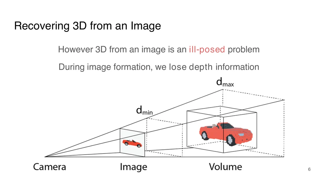
However, 3D from a single image is ill-posed: when we take a photo, the 3D scene is projected onto a 2D image plane and the depth information is lost (see Depth Ambiguity). A small car close to the camera and a large car far away can give the same image.

Slide 6: during image formation, depth is lost.

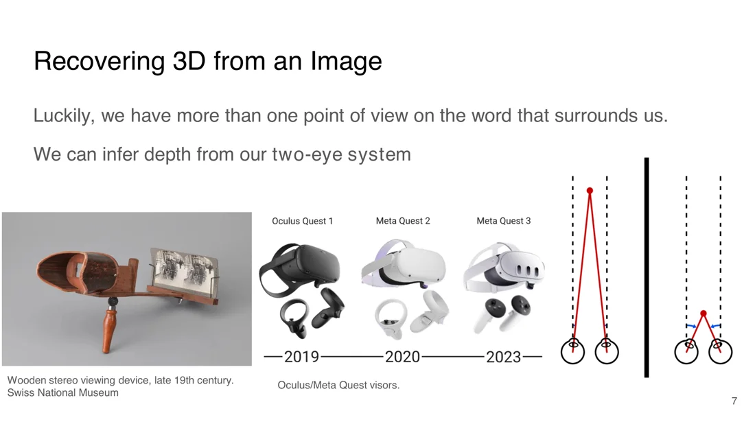
Luckily, humans have two eyes, which give two slightly different views of the world. The brain uses this difference (the disparity) to perceive depth. Stereo viewing devices were already popular in the late 19th century, and today VR/AR headsets revive the interest. We want computers to do the same: from a left and a right image, compute a depth map with the distance of every pixel.

Slide 7: we infer depth from our two-eye system.

Recap: Epipolar Geometry

Slides 9-11

(Full derivation in Lecture 3. Note that this lecture uses a slightly different notation: $p$ in image $I$, $p^{\prime }$ in image $I^{\prime }$.)

• Cameras with centers $O$ and $O^{\prime }$. The line that connects them is the baseline.
• The intersections of the image planes with the baseline are the epipoles $e,e^{\prime }$.
• If a point $p$ is observed in image $I$, the corresponding point $p^{\prime }$ must lie along the corresponding epipolar line in image $I^{\prime }$. This drastically reduces the search space.

Essential and fundamental matrix (notation of this lecture)

Canonical cameras: $p^{T}E{p}^{\prime }=0$, $E=[T_{\times }]R$

With intrinsics $K,K^{\prime }$: $p^{T}F{p}^{\prime }=0$, $F=K^{-T}E{K}^{\prime -1}$

$[T_{\times }]$ is the matrix representation of the cross product with the translation (skew-symmetric), $R$ is the rotation matrix.

Image Rectification

Slides 12-15

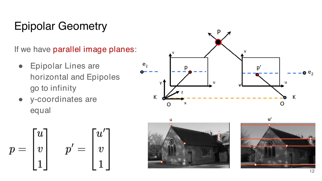
Special case: parallel image planes. Then

• the epipolar lines are horizontal and the epipoles go to infinity
• the $y$-coordinates of corresponding points are equal: $p=(u,v,1{)}^T$, $p^{\prime }=(u^{\prime },v,1{)}^T$

This simplifies stereo matching a lot, because we only search along horizontal lines.

Slide 12: with parallel image planes, epipolar lines are horizontal.

Rectification

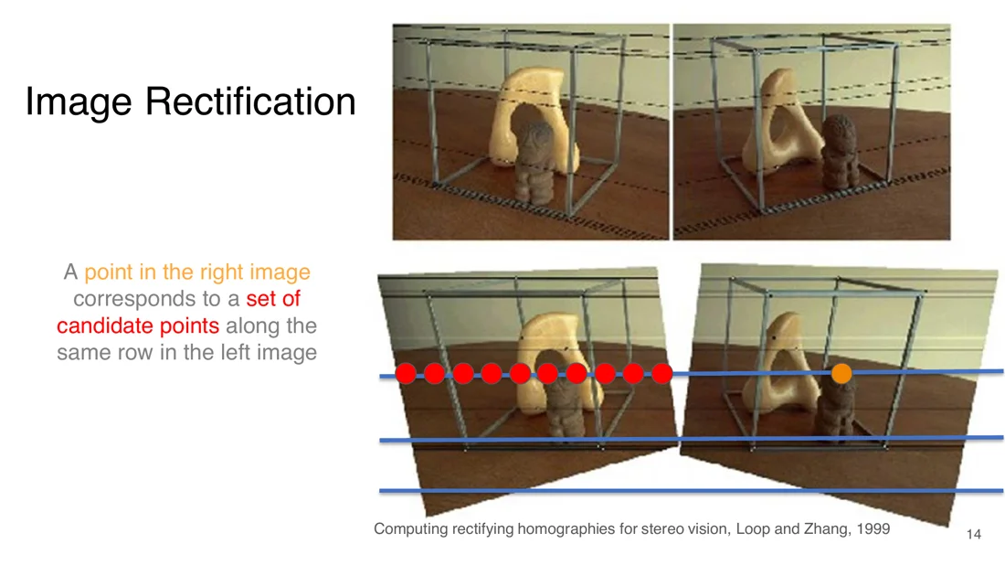
The problem of warping the camera planes to make them parallel. Existing algorithms solve it by reprojecting both image planes onto a common plane parallel to the line between the optical centers (the baseline). E.g. Computing rectifying homographies for stereo vision, Loop and Zhang, 1999.

After rectification, a point in the right image corresponds to a set of candidate points along the same row in the left image.

Slide 14: original images (top) and rectified images (bottom). The candidates lie on the same row.

After rectification, the essential matrix becomes trivial. The image planes only differ by a translation along the horizontal axis:

Essential matrix after rectification

$$R=I,t=(T,0,0),E=[t_{\times }]R=\left[\begin{array}{ccc}0& 0& 0\\ 0& 0& -T\\ 0& T& 0\end{array}\right]$$

Why this gives $v=v^{\prime }$

$$p^{T}E{p}^{\prime }=\left[\begin{array}{ccc}u& v& 1\end{array}\right]\left[\begin{array}{ccc}0& 0& 0\\ 0& 0& -T\\ 0& T& 0\end{array}\right]\left[\begin{array}{c}{u}^{\prime }\\ v^{\prime }\\ 1\end{array}\right]=\left[\begin{array}{ccc}u& v& 1\end{array}\right]\left[\begin{array}{c}0\\ -T\\ T{v}^{\prime }\end{array}\right]=-Tv+T{v}^{\prime }=0⟹v=v^{\prime }$$

Trap

Rectification is a preprocessing step. It warps the images, it does not move the cameras and does not compute depth.

Stereo Matching

Stereo matching

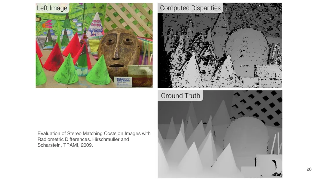
Given a pair of rectified stereo images, compute the disparity for each pixel in the reference image. The disparity is the horizontal displacement between a pair of corresponding pixels in the left and right images.

Disparity and Depth

Slides 17-19

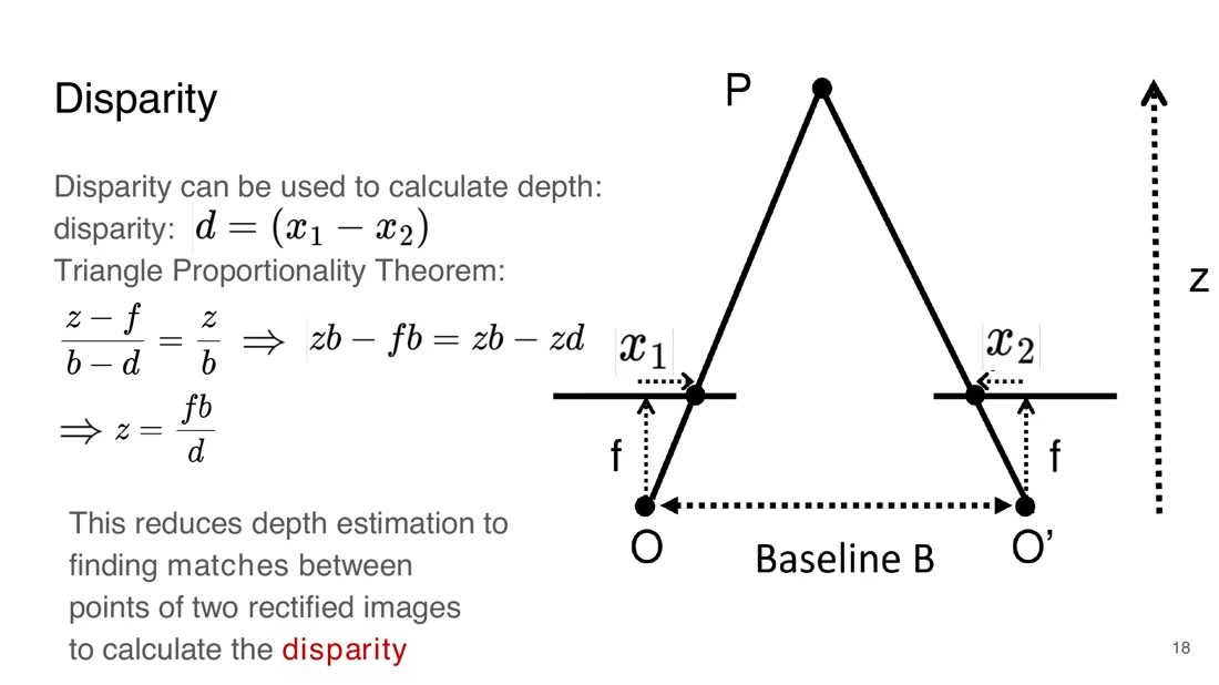
Slide 18: depth from disparity with similar triangles.

Disparity $d=x_1-x_2$, where $x_1$ is the pixel position in the left image and $x_2$ in the right. Two similar triangles: the big one from $P$ to the camera centers $O,O^{\prime }$ (base $b$, height $z$), and the small one from $P$ to the image points (base $b-d$, height $z-f$).

Depth from disparity

$$\frac{z-f}{b-d}=\frac{z}{b}⟹zb-fb=zb-zd⟹z=\frac{fb}{d}$$

$f$: focal length (pixels), $b$: baseline, $d$: disparity (pixels), $z$: depth.

Intuition

Depth is inversely proportional to disparity: close objects shift a lot between the views, far objects hardly move ($d\to 0$ means $z\to \infty$). With known $f$ and $b$, depth estimation reduces to finding matches between the two rectified images.

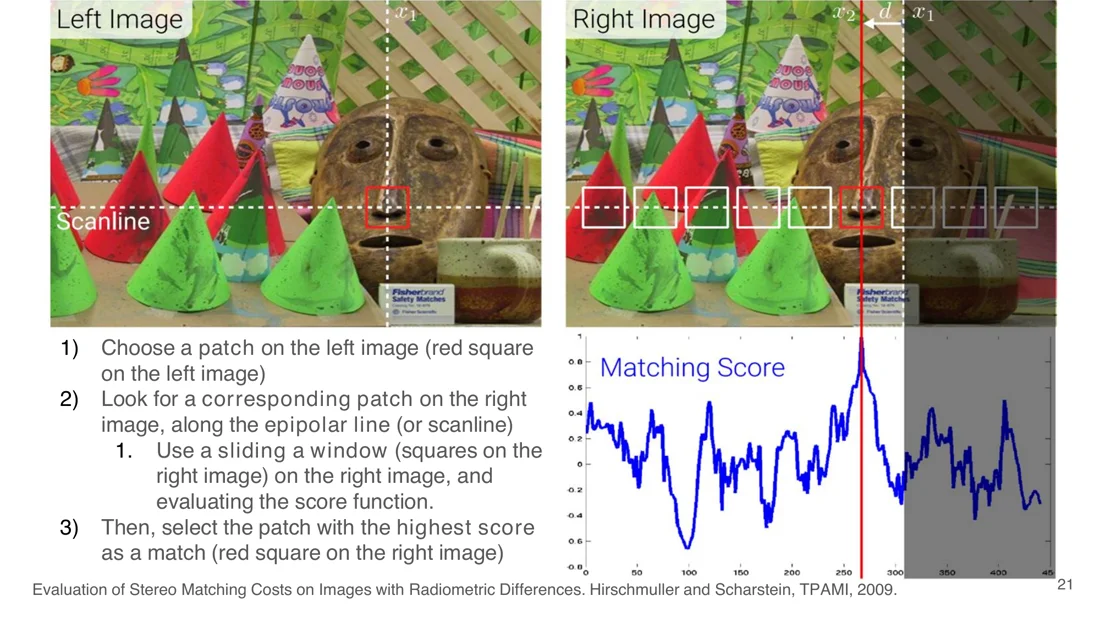
The two example images below look almost the same, but the objects are slightly shifted because of the different perspective. Because the images are rectified, corresponding pixels lie on the same scanline, so we only search horizontally.

Slide 21: sliding a window along the scanline, the matching score peaks at the correct match.

Similarity Metrics

Slides 20-22

Similarity metric approaches slide a window along the epipolar line and compute a cost with a matching / score function:

1. Choose a patch on the left image.
2. Look for the corresponding patch on the right image along the epipolar line (scanline): slide a window over the right image and evaluate the score function.
3. Select the patch with the best score as the match.

Similarity metrics

Sum of Absolute Differences:

$$\text{SAD}=\sum \left|I_L(x,y)-I_R(x-d,y)\right|$$

Sum of Squared Differences:

$$\text{SSD}=\sum {\left(I_L(x,y)-I_R(x-d,y)\right)}^2$$

Normalized Cross-Correlation:

$$\text{NCC}=\frac{\sum (I_L-{\bar{I}}_L)(I_R-{\bar{I}}_R)}{\sqrt{\sum (I_L-{\bar{I}}_L{)}^2\sum (I_R-{\bar{I}}_R{)}^2}}$$

Metric	Property
SAD	fast and easy to compute, not very robust to lighting changes
SSD	penalizes larger errors more, smoother results, but more sensitive to noise
NCC	compares the intensity patterns normalized by their variances: more robust to global illumination and contrast changes, but more expensive

Trap

SAD and SSD are costs (lower is better). NCC is a similarity (higher is better, in $[-1,1]$).

Cost Volume

Slides 23-26

For each patch of the left image, compute the metric against all patches on the corresponding epipolar line of the right image. These matching scores are the cost values.

Slide 24: for each left patch (blue), the costs against all patches on the same row of the right image (red) fill one line of the cost volume.

Cost volume

The resulting 3D volume contains the result of the cost function between each patch of the left image and each patch on the corresponding epipolar line of the right image. Its size is height × width × number of disparities (up to the image width in the simplest case). Some methods store a feature vector instead of a single cost per entry.

The cost volume is fundamental in many stereo matching pipelines, including the learned ones below.

Slide 26: computed disparities vs. ground truth.

Limitations

Slides 27-33

Handcrafted similarity functions lack flexibility and robustness:

Limitation	Why it fails
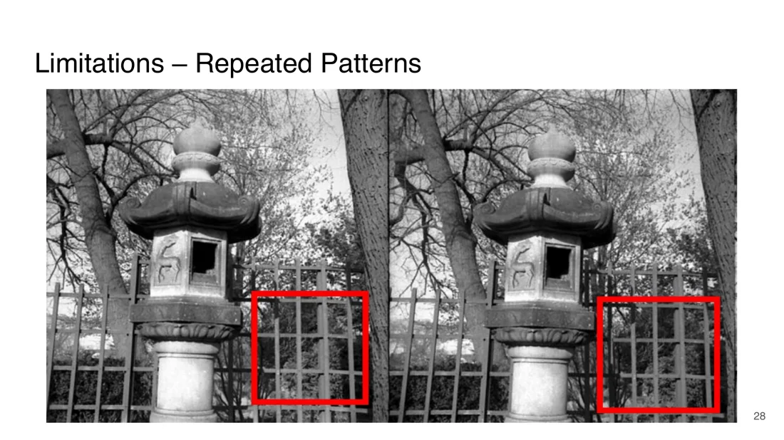
Repeated patterns	a point in the left image matches several points in the right image
Window size	too small: very sensitive to noise. Too large: smooths out details and hurts accuracy
Textureless surfaces	all patches look the same, the cost function can’t decide
Illumination change	patches look different between the views
Foreshortening (baseline)	with a short baseline, a small disparity error gives a large depth error
Occlusions	parts visible in one image are hidden in the other

Slide 28: repeated patterns

Slide 29: W = 3 vs. W = 20

Slide 30: textureless surfaces

Slide 32: foreshortening

Slide 33: occlusions

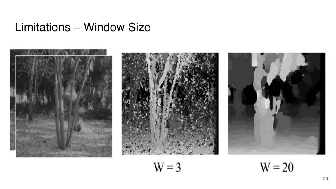
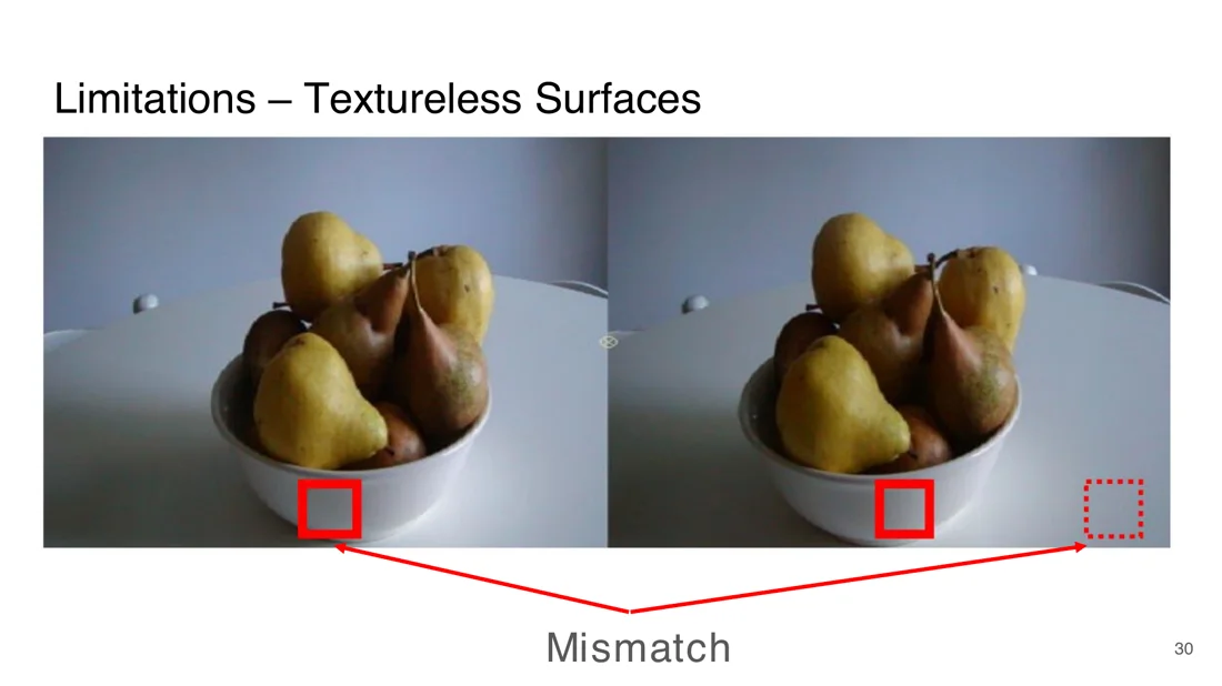
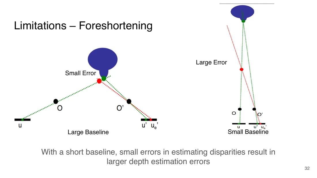
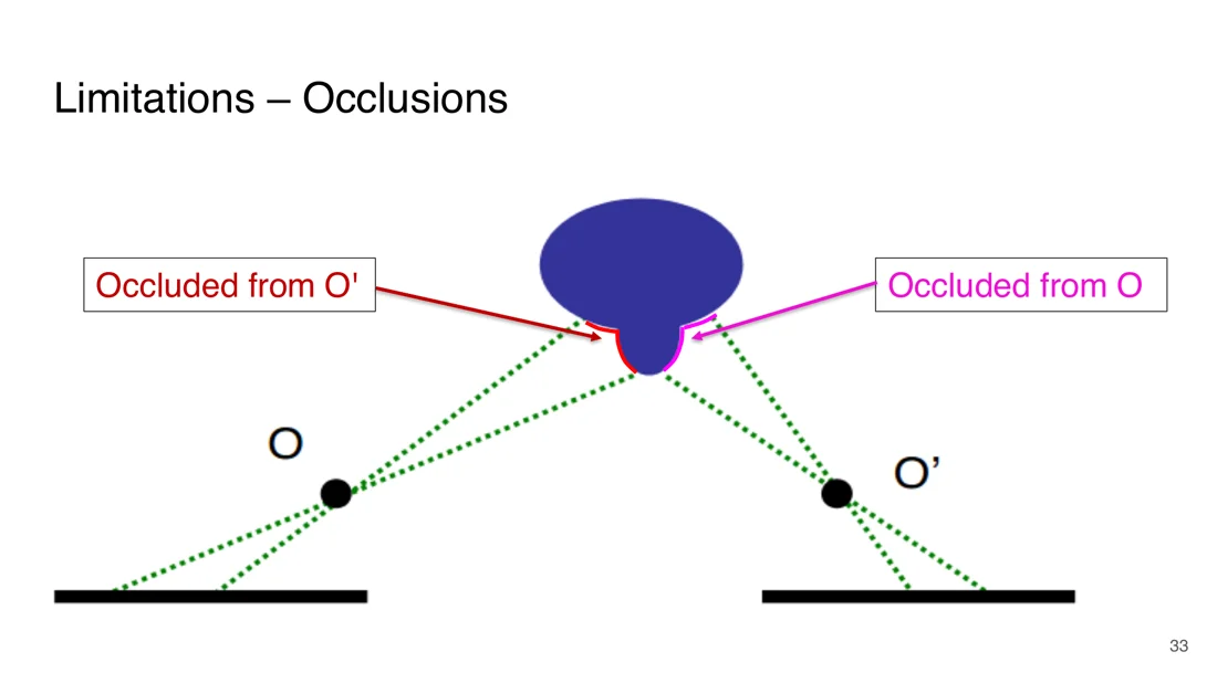
Why the baseline matters

From $z=\frac{fb}{d}$: the depth error for a disparity error $\Delta d$ is roughly $\Delta z\approx \frac{z^2}{fb}\Delta d$. A small baseline $b$ or a far point (large $z$) makes the same pixel error much worse. See Worked Examples.

Modern Stereo Matching

Slides 34-42

Today, directly evaluating cost functions on handcrafted features is not considered state of the art. Modern methods use deep learning to extract and compare features.

Learning to match windows (Siamese networks)

Slides 35-38

Zbontar and LeCun (JMLR 2016) learn the matching function instead of handcrafting it. They build a dataset of triplets:

• a reference patch from the left image
• a positive patch from the right image, whose center is the same 3D point
• a negative patch from the right image, whose center is a different 3D point

A Siamese network processes both patches with the same shared convolutional layers, concatenates the features and predicts a matching score in $[0,1]$: close to 1 for reference + positive (label 1), close to 0 for reference + negative (label 0). It is trained with a binary cross-entropy loss. For each patch we then take the best match.

Slide 36: CNN + Siamese network.

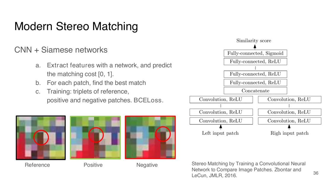
This is more robust to noise, textureless regions, repeated patterns and illumination changes, because the matching function is learned from data. It also opens the door to end-to-end pipelines.

GC-Net

Slides 39-40

GC-Net (Kendall et al., ICCV 2017) is trained end-to-end with an L1 loss between ground truth and predicted disparity. Key idea: compute a disparity cost volume and apply 3D convolutions on it.

1. Extract features with 2D convolutions (each image → feature map $H\times W\times F$).
2. Build the cost volume: for each disparity $d\in \{0,\dots ,D_{max}-1\}$, shift the right feature map horizontally by $d$ and concatenate it with the left feature map.
3. 3D convolutions aggregate matching evidence over $(H,W,D)$.
4. Predict the disparity map.

GC-Net cost volume

$$H\times W\times D_{max}\times 2F$$

$H,W$: feature map height and width. $D_{max}$: number of disparity hypotheses. $2F$: left + shifted-right features concatenated.

Slide 39: GC-Net.

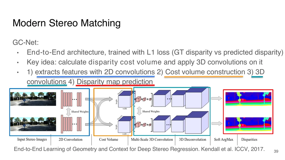
Key insight (Slide 40)

The raw features are concatenated (2F channels). The 3D convolutions learn the matching function themselves.

RAFT-Stereo

Slides 41-42

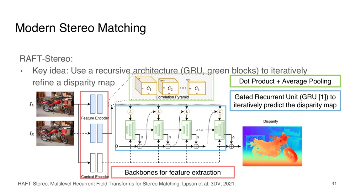
RAFT-Stereo (Lipson et al., 3DV 2021) extends RAFT (originally for optical flow). Key idea: a recurrent architecture (GRU) iteratively refines the disparity map.

1. Extract features from both images (backbones).
2. Compute the correlation between features at multiple resolutions (dot product + average pooling: a correlation pyramid).
3. A Gated Recurrent Unit updates the disparity map step by step.

This works well for occlusions, textureless regions and fine details. The disparity maps are dense and smooth, and RAFT-Stereo became a strong backbone for downstream applications.

Slide 41: RAFT-Stereo.

Slide 42: RAFT-Stereo results

Slide 42: RAFT-Stereo results

Downstream task: Stereo4D

Slides 43-45

Stereo4D (Jin et al., CVPR 2025) learns how things move in 3D from internet stereo videos.

• Input: a stereo video. Output: the movement of points in 3D (tracks).
• Key idea: extract depth with stereo matching (RAFT), the camera trajectory with SfM (COLMAP), and 2D point tracks (BootsTAP). The 2D tracks are lifted to 3D with depth and pose.

Slide 44: camera position, disparity map (from RAFT) and point tracking.

Slide 45: reconstructed dynamic 3D point clouds.

Other Applications of Rectified Images

Slides 46-51

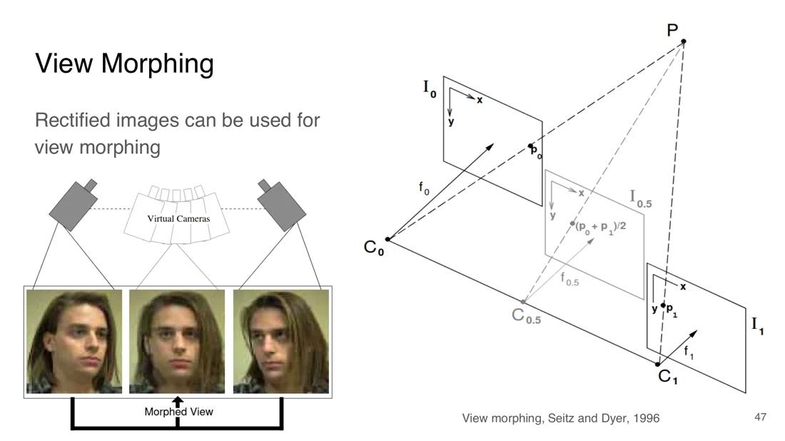
View morphing (Seitz and Dyer, 1996): from two rectified images, synthesize a novel view as if a virtual camera were placed between the two viewpoints, by interpolating geometry and appearance. Used e.g. for smooth transitions between faces.

Slide 47: view morphing.

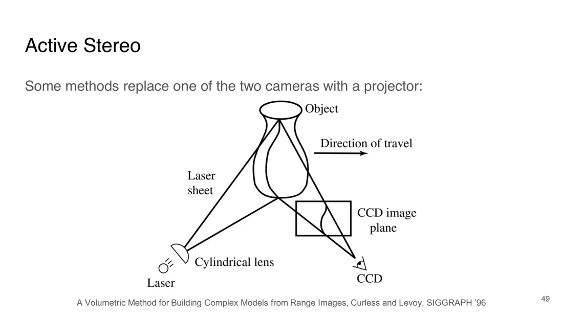
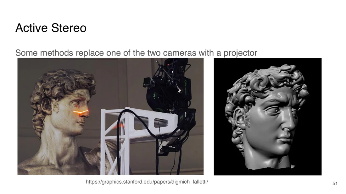
Active stereo: one of the two cameras is replaced by a projector (e.g. a laser or structured light). The light source projects a known pattern, and the camera captures how the surface geometry distorts it (Curless and Levoy, SIGGRAPH 1996). With proper calibration this gives very accurate 3D reconstructions, so it is often used to create ground truth for benchmark datasets. Famous example: the Stanford “David” scan, where a laser was swept over Michelangelo’s statue.

Slide 49: active stereo setup

Slide 51: the Digital Michelangelo project

Multi-View Stereo Matching

Slides 52-53

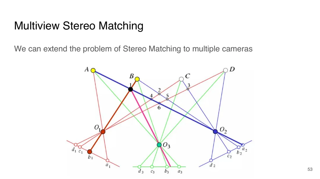
Multi-view stereo (MVS) extends stereo matching to more than two cameras. More views give more information for reconstruction, but matching now has to work across several views simultaneously. MVS needs known camera poses (e.g. from Structure from Motion) and produces a dense reconstruction.

Slide 53: stereo matching with multiple cameras.

Voxel Coloring

Slides 54-56

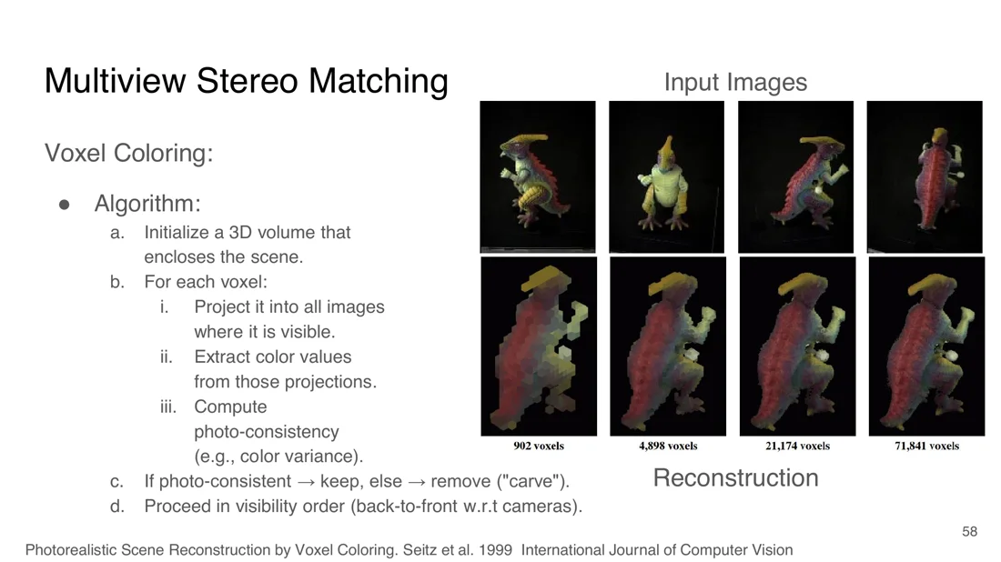
Key idea (Seitz et al., IJCV 1999): given a set of calibrated images and a grid of voxels, assign colors to the voxels so that they are consistent with all images. By carving out inconsistent voxels, we get a 3D reconstruction.

Voxel coloring algorithm

1. Initialize a 3D volume that encloses the scene.
2. For each voxel:
   • project it into all images where it is visible
   • extract the color values from those projections ($n$ colors from $n$ images)
   • compute the photo-consistency (e.g. the color variance)
3. If photo-consistent → keep (with the average color), else → remove (“carve”).
4. Proceed in visibility order (back-to-front w.r.t. the cameras).

Slide 55: voxel coloring with 902 to 71,841 voxels.

Pros	Cons
simple and intuitive	low resolution because of the voxel size
naturally handles occlusions via visibility reasoning	computationally expensive (dense grids)
no explicit feature matching needed	sensitive to calibration and lighting variation

Plane-Sweep Stereo

Slides 57-58

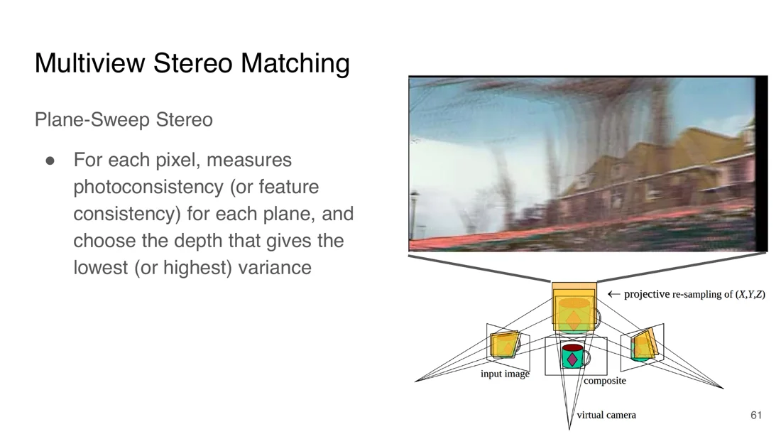
Slice the 3D scene into a series of fronto-parallel planes at different depths (parallel to the image plane of a reference/virtual camera). Project all views onto these planes using the known camera poses.

• If the depth of the plane is wrong, the projections don’t align: the overlay is blurred.
• If the depth is right, the projections align.

For each pixel, measure the photo-consistency (or feature consistency) on each plane, and choose the depth with the lowest variance (best match).

Slide 58: plane-sweep stereo.

Multi-View Stereopsis

Slides 59-60

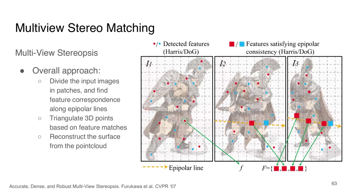
Accurate, Dense, and Robust Multi-View Stereopsis (Furukawa et al., CVPR 2007):

1. Divide the input images into patches and find feature correspondences along epipolar lines in the other views.
2. Triangulate 3D points from the feature matches.
3. Reconstruct the surface from the point cloud.

The sparse patches are densified with an iterative expand-and-filter loop: each patch proposes new patches in neighboring image regions (using its own normal and depth as initial guess), and photometric consistency across views decides whether they are kept. Finally, Poisson reconstruction turns the oriented patches into a mesh (→ Lecture 5).

Slide 60: matching along epipolar lines in multi-view stereopsis.

Modern Multi-View Stereo: MVSNet

Slides 61-67

Modern MVS uses data-driven deep learning: learn the feature representations and matching functions from data instead of hand-designing them.

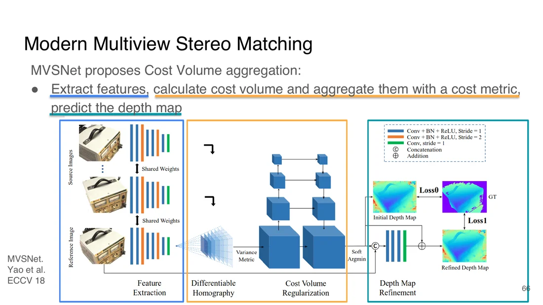
MVSNet (Yao et al., ECCV 2018): extract features, build a cost volume, aggregate it with a cost metric, predict the depth map.

• Extract features from each input image.
• Plane sweep with a differentiable homography: for each of the $D$ depth levels, warp the source view features into the reference camera’s frustum.
• Aggregate the warped features across all views with the variance, which gives a cost volume aligned with the reference image.
• Regularize the cost volume (3D CNN) and predict an initial depth map, then refine it.

Slide 63: MVSNet.

Cost volume: stereo vs. multi-view (Slide 64)

	GC-Net (rectified stereo)	MVSNet (multi-view)
Hypothesis	disparity $d\in \{0,\dots ,D_{max}-1\}$	depth $z\in \{z_1,\dots ,z_D\}$ along reference rays
Align views by	horizontal pixel shift (trivial, works only because the images are rectified)	differentiable homography (plane sweep: warp each source view onto a depth plane)
Combine features	concatenate left + shifted right: $2F$ channels, locked to 2 views	variance across $N$ views: $F$ channels, independent of $N$. Low variance ⇒ good match
Volume shape	$H\times W\times D_{max}\times 2F$	$H\times W\times D\times F$

Same idea (4D tensor + 3D convolutions), but the hypothesis axis changes: stereo hypothesizes disparities (1D shifts along a scanline), multi-view hypothesizes depths (planes in 3D), which is needed when cameras have arbitrary poses.

Further reading: MVSAnywhere (CVPR 2025), Stereo Anywhere (CVPR 2025), Selective-Stereo (CVPR 2024), Cross-spectral Gated-RGB Stereo (CVPR 2024), MoCha-Stereo (CVPR 2024).

Teaser: current methods like VGGT (Visual Geometry Grounded Transformer, CVPR 2025) reconstruct complete 3D scenes (cameras, depths, points, correspondences) from unposed images in a single forward pass, without any of the math above (→ Lecture 9).

Monocular Depth Estimation

Slides 68-70

Monocular depth estimation

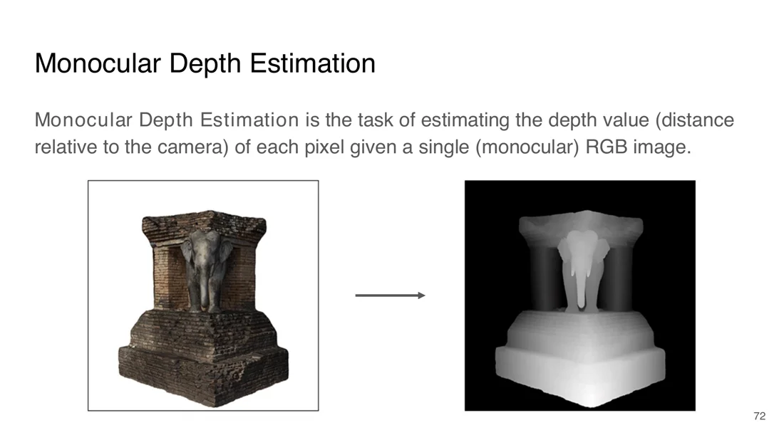
Estimate the depth value (distance relative to the camera) of each pixel given a single (monocular) RGB image.

Recent deep learning advances made it possible (interest grew strongly in recent years). The reason: we now learn depth from data with direct supervision, thanks to three factors: data, architecture, training objective.

Slide 69: monocular depth estimation.

Data, Architecture, Training Objective

Slides 71-76

Data:

• Real-world data: cheap depth sensors made it possible, e.g. the Microsoft Kinect (stereo sensors, Time-of-Flight sensors, structured light / IR). Example: NYU Depth V2 (Silberman et al., ECCV 2012).
• Synthetic data: realistic game engines and synthetic scenes generate large labeled datasets in a controlled way (e.g. Rajpal et al., CVPR 2023).

Architecture: CNNs, GANs, diffusion models… Architectures evolved dramatically, and the number of parameters grew from millions to billions today.

Training objective: a simple objective lowers the error between prediction and ground truth. Given an image $x$ and the predicted depth $y=f(x)$:

Simple training objective

$$\mathcal{L}(y,\hat{y})=\sum _i\Vert y_i-{\hat{y}}_i{\Vert }^2,y=f(x)$$

($\hat{y}$ is the ground truth depth on the slides.)

The Problem: Scale / Depth Ambiguity

Slides 77-80

Monocular depth estimation is ill-posed: a small, close object looks exactly the same as a larger, farther-away object. Absolute scale and depth are ambiguous from a single image.

Slide 77: scale / depth ambiguity.

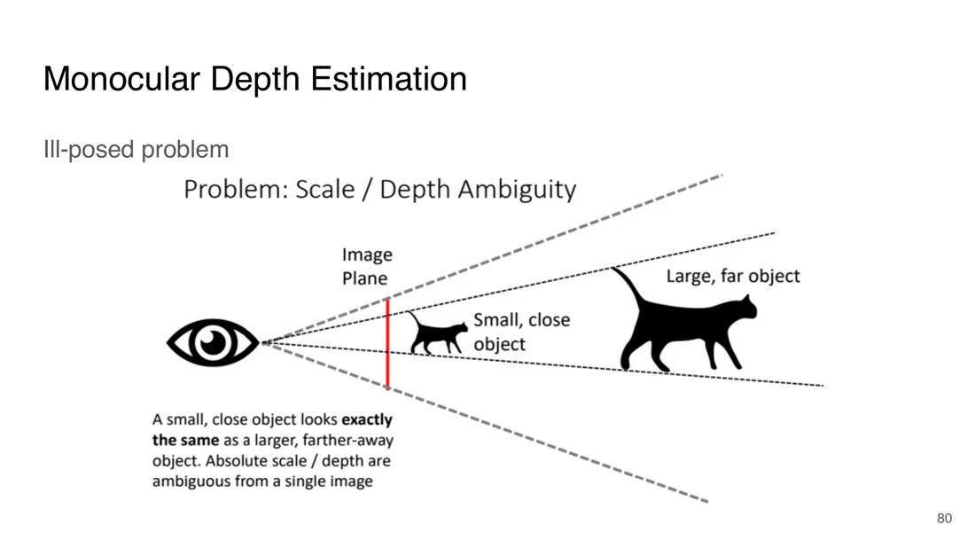
Sometimes we can fight back: use a loss that is invariant to the global scale. It uses the mean depth to measure the relationship between points instead of their absolute value.

Scale-invariant mean squared error (Eigen, Puhrsch and Fergus, NeurIPS 2014)

$$\mathcal{L}(y,\hat{y})=\sum _i{\Vert \log y_i-\log {\hat{y}}_i+\alpha (y,\hat{y})\Vert }^2,\alpha (y,\hat{y})=\frac{1}{n}\sum _i\left(\log {\hat{y}}_i-\log y_i\right)$$

Why log space?

If the output is off by a multiplicative constant, $y=s\cdot \hat{y}$, then in log space $\log y-\log \hat{y}=\log s$. This is constant across all pixels, and $\alpha$ is exactly $-\log s$, so it cancels. The loss ignores the global scale.

But we cannot do magic: sometimes the visual evidence is not enough. Depth Anything V2 (a state-of-the-art model) completely fails on the Ames room illusion.

Slide 80: the Ames room illusion (also in Lecture 1).

To improve monocular depth estimation: acquire more data, improve the network architecture, formulate better training objectives. It is a very active field: new methods appear every month (e.g. ZoeDepth, Depth Anything v1/v2, UniDepth, Marigold, Depth Pro).

Limitations of Supervised Data

Slides 83-85

Real labeled depth data is limited in quantity and quality:

• Quantity: annotation doesn’t scale. Capturing accurate depth needs complex rigs (e.g. LiDAR rigs on cars).
• Quality: sensor and algorithm failures.
  • Time-of-Flight sensors like the Kinect are noisy near transparent and absorbent materials.
  • Stereo-matching labels (e.g. HR-WSI, 2020) are noisy on repetitive patterns.
  • SfM-based labels (e.g. MegaDepth) are wrong on dynamic objects.
  • Deep networks handle random noise well, but these systematic errors show up in the trained models.

Slide 84: label noise in real depth datasets.

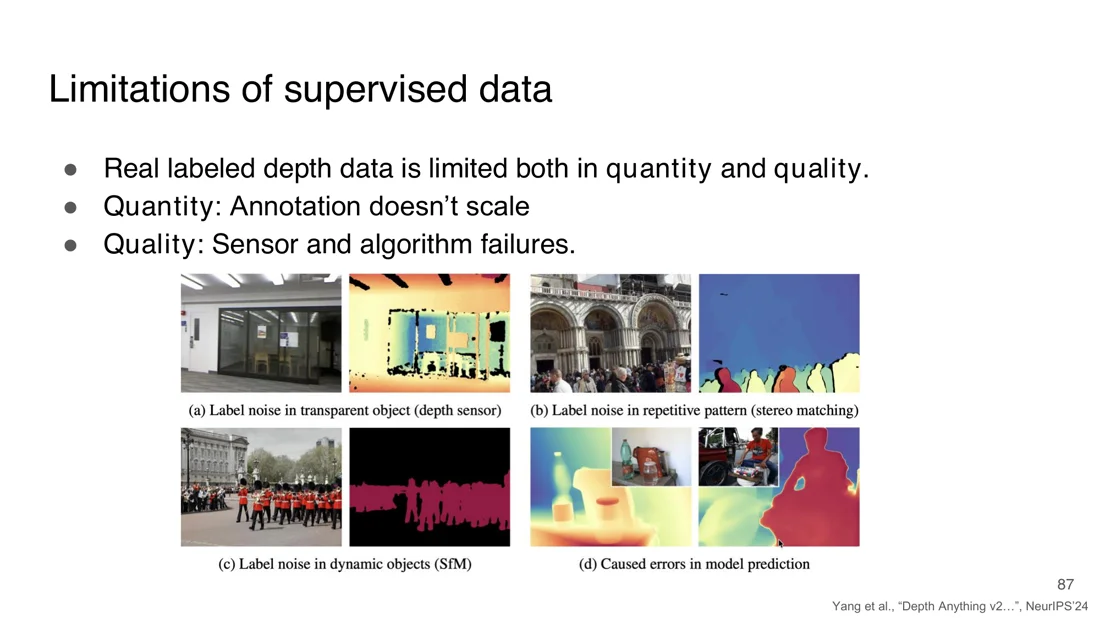
Solution: semi-supervised learning. Train on high-quality data only, then learn from unlabeled images.

Depth Anything

Slides 86-88

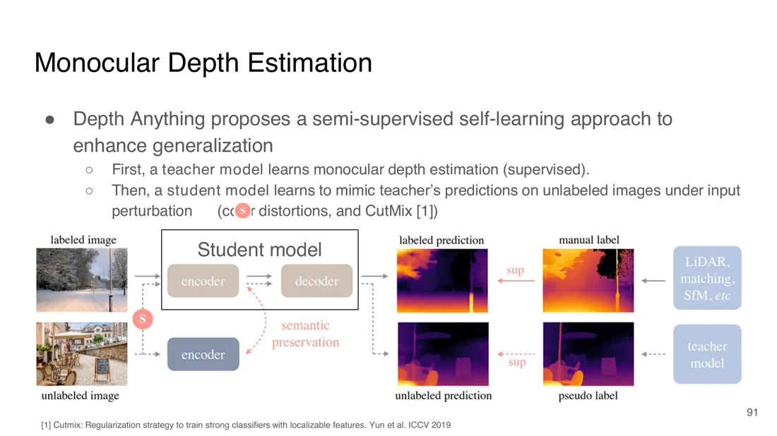
Depth Anything proposes a semi-supervised self-learning approach to improve generalization, because most images online have no depth labels:

1. A large teacher model (encoder + decoder) learns monocular depth estimation supervised on labeled data (LiDAR, matching, SfM, …).
2. A student model learns to mimic the teacher’s predictions (pseudo labels) on unlabeled images under input perturbations: color distortions and CutMix (randomly cutting and mixing patches of different images). A semantic preservation term keeps its features close to a frozen encoder.

The perturbations force the student to learn the essential, invariant features, which according to the authors is the key to better generalization.

Slide 88: teacher-student training in Depth Anything.

Feature Extraction Backbones

Slides 89-90

Large pre-trained backbones that were not trained for depth are excellent feature extractors and can be adapted:

• DINOv2 (Meta): trained for general-purpose image understanding, adapted for depth estimation with results comparable to the state of the art.
• ViT (Vision Transformer) for dense prediction (DPT, Ranftl et al., ICCV 2021).

Conclusions

Slides 91-92

• Stereo matching computes disparity maps from two images. Depth follows from the disparity.
• We saw classical and recent methods for disparity computation.
• Multi-view stereo extends this to many views: reconstruct geometry and predict depth.
• Monocular depth estimation, with current state-of-the-art methods that use large models, better training objectives and new data strategies.

	Stereo	Multi-view stereo	Monocular
Views	2 (rectified)	$N$ with known poses	1
Hypothesis	disparity $d$	depth $z$ / voxel	none (direct regression)
Depth comes from	$z=fb/d$	consistency across $N$ views	a prior learned from data
Classical	sliding window + SAD / SSD / NCC	voxel coloring, plane sweep, multi-view stereopsis	none
Learned	Siamese CNN, GC-Net, RAFT-Stereo	MVSNet	Depth Anything, DINOv2 / ViT backbones

Worked Examples

Example 1: depth from disparity

Rectified stereo camera with focal length $f=700$ px and baseline $b=0.1$ m. A point has $x_1=420$ px in the left and $x_2=406$ px in the right image.

$$d=x_1-x_2=14\text{ px},z=\frac{fb}{d}=\frac{700\cdot 0.1}{14}=5\text{ m}$$

Example 2: why the baseline matters (1 px disparity error)

$f=700$ px. The true depth is $z$, the disparity is off by 1 px.

Baseline $b$	true $z$	true $d=fb/z$	$d$ with 1 px error	estimated $z$	error
0.1 m	5 m	14 px	13 px	5.38 m	38 cm
0.5 m	5 m	70 px	69 px	5.07 m	7 cm
0.1 m	10 m	7 px	6 px	11.67 m	1.67 m

Short baseline and far points give large depth errors (roughly $\Delta z\approx \frac{z^2}{fb}\Delta d$). A large baseline reduces the error, but causes more occlusions and stronger appearance differences between the views.

Exam relevance

Stereo was not among the remembered exam tasks, but it lies in the gap of forgotten tasks (lectures 3-6), and it is multiple-choice material. Know:

• rectification: what it does and why the essential matrix becomes trivial
• $d=x_1-x_2$ and $z=\frac{fb}{d}$ (derivation with similar triangles), and why a short baseline is bad
• SAD, SSD, NCC and their properties
• the cost volume and the limitations of classical stereo
• GC-Net vs. MVSNet cost volumes
• monocular depth: data / architecture / training objective, the scale-invariant loss and why it works in log space

Self-Test

What does rectification do, and what does the essential matrix look like afterwards?

Answer $y$. Then $R=I$, $t=(T,0,0)$ and $E=[t_{\times }]=\left[\begin{array}{ccc}0& 0& 0\\ 0& 0& -T\\ 0& T& 0\end{array}\right]$.

It warps both images onto a common plane parallel to the baseline. Epipolar lines become horizontal, epipoles go to infinity, corresponding points have the same

Derive the depth from the disparity.

Answer $\frac{z-f}{b-d}=\frac{z}{b}$, so $zb-fb=zb-zd$ and $z=\frac{fb}{d}$ with $d=x_1-x_2$.

Similar triangles:

Compare SAD, SSD and NCC.

Answer

SAD: sum of absolute differences, fast, not robust to lighting. SSD: sum of squared differences, penalizes large errors more, more sensitive to noise. NCC: normalized cross-correlation, robust to global illumination and contrast changes, but more expensive. SAD/SSD are costs (lower is better), NCC a similarity (higher is better).

What is a cost volume?

Answer $H\times W\times D_{max}\times 2F$).

The 3D volume (height × width × number of disparities) of matching costs between every left patch and every candidate patch on the corresponding scanline of the right image. Learned methods store feature vectors instead (e.g. GC-Net:

Name the limitations of classical stereo matching.

Answer

Repeated patterns, window size trade-off (noise vs. smoothing), textureless surfaces, illumination changes, foreshortening (short baseline → large depth error), occlusions.

How does the Siamese network of Zbontar and LeCun learn matching?

Answer $[0,1]$ (1 for reference + positive, 0 for reference + negative), trained with binary cross-entropy.

Triplets of reference, positive and negative patches. Shared convolutional layers on both patches, then fully connected layers predict a score in

What is the key idea of GC-Net and of RAFT-Stereo?

Answer

GC-Net: build a 4D cost volume by concatenating left and shifted-right features for each disparity, apply 3D convolutions, train end-to-end with an L1 loss. RAFT-Stereo: multi-resolution correlation of features, and a GRU iteratively refines the disparity map.

Explain voxel coloring and plane-sweep stereo.

Answer

Voxel coloring: project each voxel into all images where it is visible, keep it if the colors are consistent (low variance), carve it otherwise, in visibility order. Plane sweep: project all views onto fronto-parallel planes at different depths; for each pixel choose the depth where the projections agree best (lowest variance).

How does the MVSNet cost volume differ from the GC-Net cost volume?

Answer $2F$ channels). MVSNet hypothesizes depths along the reference rays, warps the source views with a differentiable homography and combines $N$ views with the variance ($F$ channels, independent of $N$).

GC-Net hypothesizes disparities (horizontal shifts, rectified pair) and concatenates 2 views (

Why is monocular depth estimation ill-posed, and how does the scale-invariant loss help?

Answer $\alpha$; a global scale factor $s$ becomes the constant $\log s$ in log space and cancels.

A small close object looks like a large far one, so the absolute scale is ambiguous. The loss compares log depths and subtracts the mean log difference

How does Depth Anything use unlabeled images?

Answer

A teacher is trained supervised on labeled data. A student learns to reproduce the teacher’s predictions (pseudo labels) on unlabeled images under perturbations (color distortions, CutMix), which improves generalization.

Related

• Previous: Lecture 3: Classical Reconstruction · Next: Lecture 5: Surface Reconstruction · Course: Overview
• Concepts: Image Rectification, Disparity, Stereo Matching, Cost Volume, Multi-View Stereo, Monocular Depth Estimation, Epipolar Geometry, Depth Ambiguity
• The simple stereo camera model was introduced in Lecture 2.1.