Lecture 8: 3D Gaussian Splatting

TL;DR

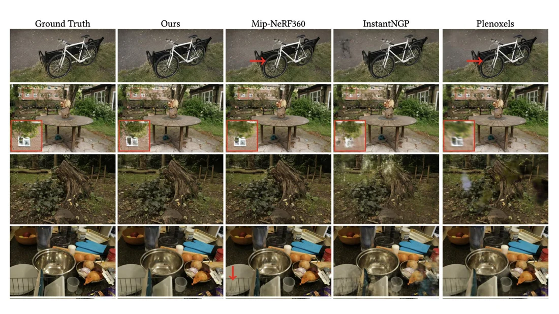
1. NeRF is slow because it queries an MLP for every sample along every ray. 3D Gaussian Splatting (Kerbl & Kopanas et al., SIGGRAPH 2023) represents the scene explicitly by millions of 3D Gaussians, without any neural network.
2. Each Gaussian has a mean $\mu$, a covariance $\Sigma =RS{S}^T{R}^T$ (rotation as a quaternion + 3 scales, so it always stays valid), an opacity $o$ and a color (RGB or spherical harmonics).
3. To render, the Gaussians are projected to 2D (${\Sigma }^{\prime }=JW\Sigma W^T{J}^T$), sorted by depth and alpha-blended: $C={\sum }_i{\mathbf{c}}_i{\alpha }_i{\prod }_{j<i}(1-{\alpha }_j)$ with ${\alpha }_i=o_i{G}_i^{2D}(\mathbf{x})$. The same image formation as NeRF, only $\alpha$ is computed differently.
4. Real time through GPU rasterization: $16\times 16$ tiles and one global depth sort. Training: initialize from SfM points, optimize with an $L_1$ + D-SSIM loss, and clone / split Gaussians (adaptive density control).
5. Limitations and follow-ups: high storage → compression (EAGLES); static scenes → Dynamic 3D Gaussians; no clean surface → SuGaR.

Exam relevance

Exam task 4: the NeRF and 3DGS rendering formulas were given; explain every symbol and compare the two. See Image Formation: NeRF vs. 3D Gaussian Splatting and the full comparison in Lecture 7.

Outline: problems of NeRF · point-based rendering · 3D Gaussian Splatting · applications and limitations (dynamic scenes, compression, surface reconstruction).

Problems of NeRF

Slide 3

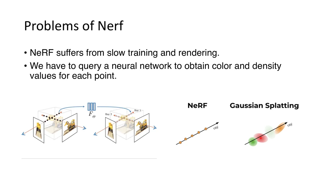
• NeRF suffers from slow training and rendering.
• We have to query a neural network to get color and density for each point sampled along each ray.

Gaussian splatting instead places a few explicit primitives along the ray.

Slide 3: NeRF (many MLP queries per ray) vs. Gaussian Splatting (a few explicit Gaussians).

Point-Based Rendering

Slides 4-6

One way around NeRF is to revisit point-based rendering, which is based on alpha blending: the color of a pixel is a blended combination of the colors of the points that fall into that pixel.

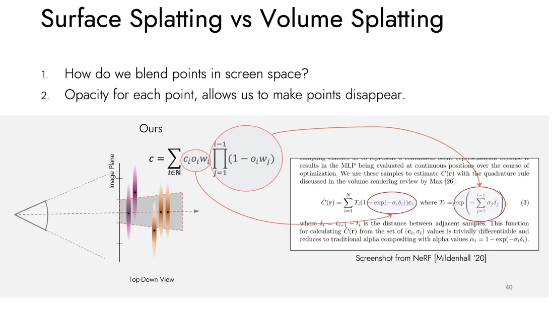
Surface splatting vs. volume splatting

How do we blend points in screen space?

$$\text{Surface splatting (normalized weights): }c=\frac{{\sum }_{i\in \mathcal{N}}{c}_i{w}_i}{{\sum }_{i\in \mathcal{N}}{w}_i}\text{Volume splatting (ordered blending): }c=\sum _{i\in \mathcal{N}}{c}_i{w}_i\prod _{j=1}^{i-1}(1-w_j)$$

Opacity for each point allows us to make points disappear:

$$\text{3DGS: }c=\sum _{i\in \mathcal{N}}{c}_i{o}_i{w}_i\prod _{j=1}^{i-1}(1-o_j{w}_j)$$

$w_i$: how much of the pixel the (projected) Gaussian covers; $o_i$: how visible the Gaussian’s color is.

	Surface splatting	Volume splatting
Input data	point cloud (surface)	volumetric grid / voxel data
Rendering target	visible surfaces only	the full 3D volume, including internal structures
Appearance	opaque surfaces	translucent effects (fog, tissue, gas, clouds)
Projection	oriented disks or elliptical Gaussians	spherical or isotropic kernels
Compositing	often depth-buffer based	alpha blending with accumulation along rays
Use case	real-time surface rendering	medical / scientific volume visualization

Slide 6: the 3DGS blending formula next to NeRF's. The product is the transmittance (probability that Gaussian i is not occluded).

Why not use $w_i$ alone as opacity?

$w_i$ is purely view-dependent: it changes with the camera angle and distance. The opacity $o_i$ is learned and view-independent: it encodes density, material (glass vs. wood) and boundaries. Separating the two makes the model more expressive (semi-transparency, fade-outs) and helps with correct compositing and anti-aliasing.

3D Gaussian Splatting

Goal and Overview

Slides 7-10

Goal: given images or videos and their camera poses, reconstruct the 3D world, and then render it from new (ideally unseen) views at high speed: novel view synthesis.

Slide 8: a scene reconstructed with 3DGS, explored from new views in real time.

3D Gaussian Splatting (Kerbl & Kopanas et al., 2023)

• a splat-based representation
• uses 3D Gaussians instead of points or a mesh (unlike points, Gaussians have a volume)
• does not include any neural network

flowchart LR
  S["SfM points<br/>(COLMAP)"] --> I["Initialization"] --> G["3D Gaussians"]
  G --> P["Projection<br/>(camera)"] --> R["Differentiable<br/>tile rasterizer"] --> IMG["Image"]
  IMG -. "gradient flow" .-> G
  G <--> A["Adaptive density<br/>control"]

Slide 10: method overview.

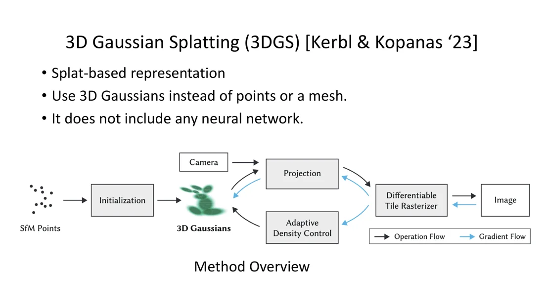
Initialization: run an SfM method (e.g. COLMAP) on the images. The SfM points give the 3D positions of the first Gaussians, optionally with a color.

Parametrization of a 3D Gaussian

Slides 11-12

Parameters of one 3D Gaussian

• mean $\mu$: the position $(x,y,z)$
• covariance $\Sigma$: shape and orientation of the ellipsoid
• opacity $o$: a sigmoid maps the parameter to $[0,1]$
• color $\mathbf{c}$: 3 values (RGB) or spherical harmonics (SH) coefficients (view-dependent color)

$$G(\mathbf{x})=\exp \left(-\frac{1}{2}(\mathbf{x}-\mu {)}^T{\Sigma }^{-1}(\mathbf{x}-\mu )\right)$$

How to Optimize the Covariance Matrix

Slides 13-14

A 3D Gaussian can be an ellipsoid rotated and stretched in any direction. Why not optimize the 9 entries of $\Sigma$ directly?

• Not all symmetric matrices are covariance matrices, and gradient updates can easily make them invalid.
• $\Sigma$ describes the configuration of an ellipsoid; it only has a physical meaning if it is positive semi-definite. This constraint is hard to enforce with gradient descent.

So we factorize it:

Covariance from rotation and scale

$$\Sigma =RS{S}^T{R}^T$$

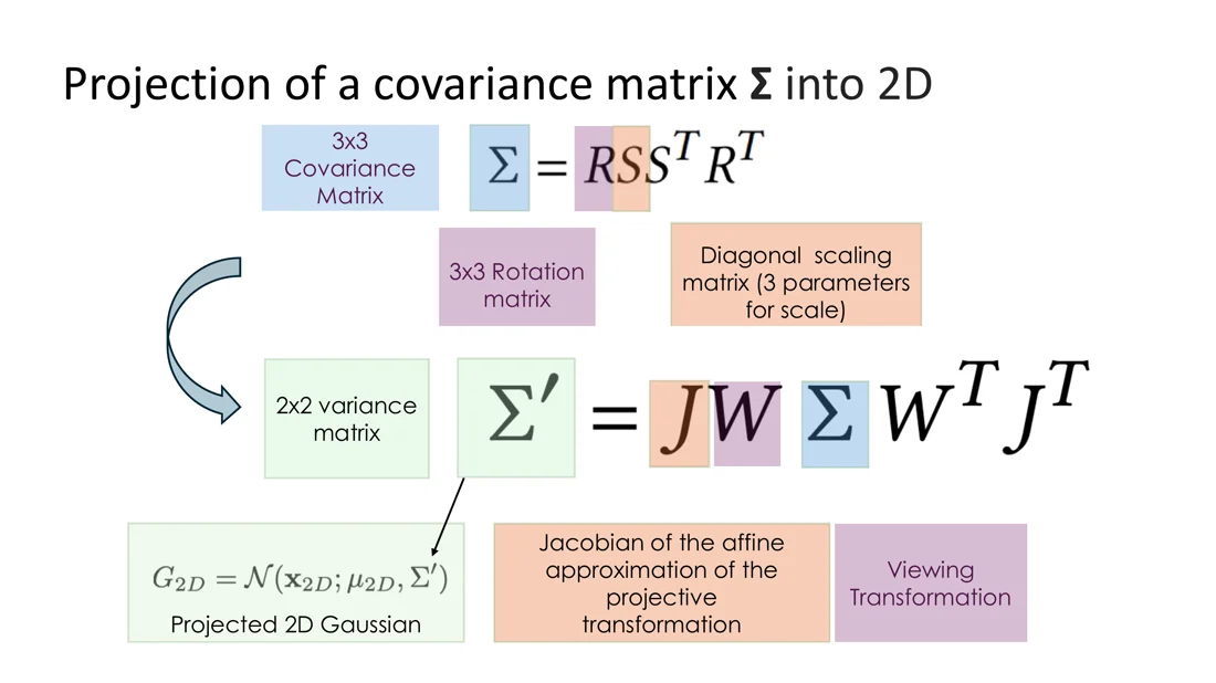
$S$: diagonal scaling matrix (3 parameters). $R$: $3\times 3$ rotation matrix, expressed analytically by a quaternion (4 parameters). This is the eigendecomposition of a covariance matrix; the result is always a valid (rotated, stretched) ellipsoid.

(Rotations as quaternions: Lecture 2.2.)

Projection of the Covariance into 2D

Slides 15-16

Projected 2D Gaussian

$${\Sigma }^{\prime }=JW\Sigma W^T{J}^T,G_{2D}=\mathcal{N}({\mathbf{x}}_{2D};{\mu }_{2D},{\Sigma }^{\prime })$$

$W$: viewing transformation (world → camera). $J$: Jacobian of the affine approximation of the projective transformation. ${\Sigma }^{\prime }$: the resulting $2\times 2$ covariance on the image plane (from the $3\times 3$ result, the third row and column are dropped).

Slide 16: projection of the covariance matrix into 2D.

Intuition

Perspective projection is not linear (division by $Z$, see Lecture 2.1), so a projected Gaussian would not be a Gaussian anymore. Linearizing the projection around the Gaussian’s center (the Jacobian $J$) keeps it Gaussian, and the 2D covariance can be computed in closed form.

Image Formation: NeRF vs. 3D Gaussian Splatting

Slides 17-19

Point-based $\alpha$-blending and NeRF-style volume rendering share essentially the same image formation model.

NeRF (Slide 17)

$$C=\sum _{i=1}^N{T}_i{\alpha }_i{\mathbf{c}}_i,{\alpha }_i=1-\exp (-{\sigma }_i{\delta }_i),T_i=\prod _{j=1}^{i-1}(1-{\alpha }_j)$$

Samples along the ray through the pixel, with density ${\sigma }_i$ and color ${\mathbf{c}}_i$ from the MLP and intervals ${\delta }_i$.

3D Gaussian Splatting (Slide 18)

$$C=\sum _{i\in \mathcal{N}}{\mathbf{c}}_i{\alpha }_i\prod _{j=1}^{i-1}(1-{\alpha }_j),{\alpha }_i=o_i{G}_i^{2D}(\mathbf{x})$$

Blending the $\mathcal{N}$ depth-ordered Gaussians that overlap the pixel $\mathbf{x}$.

Symbol	Meaning
$C$	color of the pixel
$i\in \mathcal{N}$	the Gaussians overlapping the pixel, sorted front to back
${\mathbf{c}}_i$	color of Gaussian $i$ (from its spherical harmonics and the viewing direction)
$o_i$	learned opacity of Gaussian $i$
$G_i^{2D}(\mathbf{x})$	the projected 2D Gaussian (mean ${\mu }_{2D}$, covariance ${\Sigma }^{\prime }$) evaluated at the pixel $\mathbf{x}$
${\alpha }_i=o_i{G}_i^{2D}(\mathbf{x})$	how much Gaussian $i$ contributes at this pixel
${\prod }_{j=1}^{i-1}(1-{\alpha }_j)$	transmittance: probability that Gaussian $i$ is not occluded by the Gaussians in front

Slide 19: the image formation model is the same; only α differs.

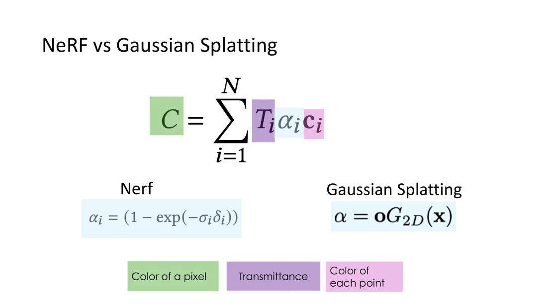
Same formula, drastically different speed

The only difference in the equations is how $\alpha$ is computed. In practice it matters enormously:

• NeRF is a continuous, implicit representation of empty/occupied space. Finding the samples needs expensive random sampling along each ray, with noise and heavy compute.
• Points (Gaussians) are an unstructured, discrete, explicit representation, still flexible enough to create, destroy and move geometry. Each pixel aggregates an ordered list of projected 2D Gaussians.

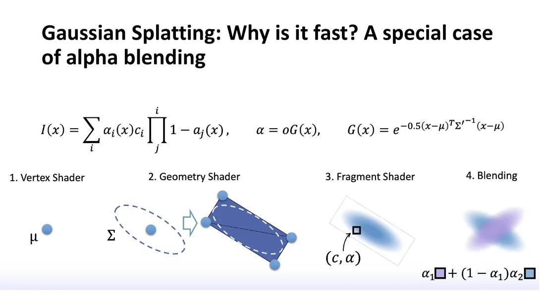
Why Is It Fast? A Special Case of Alpha Blending

Slides 20-21, 25-26

$$I(\mathbf{x})=\sum _i{\alpha }_i(\mathbf{x}){\mathbf{c}}_i\prod _{j<i}(1-{\alpha }_j(\mathbf{x})),\alpha =oG(\mathbf{x}),G(\mathbf{x})=e^{-0.5(\mathbf{x}-\mu {)}^T{\Sigma }^{\prime -1}(\mathbf{x}-\mu )}$$

This maps directly onto the GPU graphics pipeline, which runs massively in parallel:

Stage	For 3DGS	Runs
1. Vertex shader	transform the center $\mu$ to screen space	per vertex
2. Geometry shader	build a screen-space quad around the ellipse ${\Sigma }^{\prime }$	per primitive
3. Fragment shader	evaluate $(\mathbf{c},\alpha )$ for every covered pixel	per fragment
4. Blending	${\alpha }_1{\mathbf{c}}_1+(1-{\alpha }_1){\alpha }_2{\mathbf{c}}_2+\dots$	per pixel

Slide 20: Gaussian splatting as a special case of alpha blending on the GPU.

Slide 21: the rendering (left) and the underlying 3D Gaussians (right).

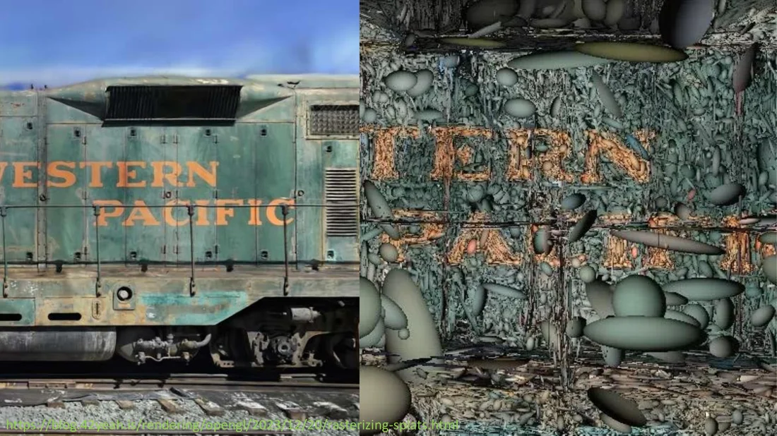
How to go from 5 FPS to 100+ FPS (using the GPU efficiently):

1. Tiling: split the image into $16\times 16$ tiles, so threads can work together. Each Gaussian is only checked against the tiles it overlaps, not against every pixel; much less overdraw.
2. Single global sort: instead of sorting per tile or per pixel, sort all visible Gaussians once by depth (GPUs sort millions of primitives fast). Each tile then streams the sorted list and takes only the Gaussians that intersect it.

flowchart LR
  A["project all 3D Gaussians<br/>to 2D (screen bounds)"] --> B["one global<br/>depth sort"] --> C["assign Gaussians<br/>to 16×16 tiles"] --> D["render each tile<br/>independently, in parallel"]

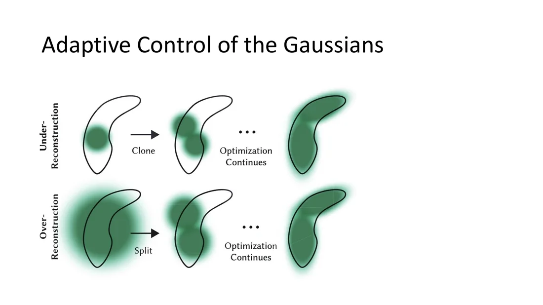
Adaptive Control of the Gaussians

Slides 21-23

The SfM initialization only gives a sparse point cloud, but scenes are dense. So 3DGS adaptively controls the number of Gaussians during optimization:

• Under-reconstruction (small geometry is insufficiently covered): clone the Gaussian.
• Over-reconstruction (small geometry is covered by one large splat): split it into two.

Slide 23: adaptive density control.

Optimization

Slides 24-29

The Gaussians are optimized so that renders of the scene closely match the known dataset images:

Loss

$$\mathcal{L}=(1-\lambda ){\mathcal{L}}_1+\lambda {\mathcal{L}}_{\text{D-SSIM}}$$

${\mathcal{L}}_1$ between the rendered and the ground-truth image, plus a structural similarity term (D-SSIM). Gradients flow back through the differentiable rasterizer to all Gaussian parameters.

Slide 27: real-time rendering of a 3DGS scene

Slide 28: the bicycle scene

Slide 29: 3DGS vs. Mip-NeRF360, Instant NGP and Plenoxels on held-out views.

Limitations and Follow-Up Works

Slides 30-33

Limitation	Follow-up
High storage cost	compression (e.g. EAGLES)
Novel view synthesis of mostly static scenes	extending to dynamic scenes (Dynamic 3DGS)
Unlike meshes, no clean / compact surface	surface reconstruction (e.g. SuGaR)

Storage Cost and Compression

Slides 34-38

One Gaussian needs 59 × 4 bytes: mean (3) + scale (3) + rotation (4) + SH color (16 × 3 = 48) + opacity (1) = 59 floats. A scene has millions of them.

Slide 34: storage cost of a 3DGS scene.

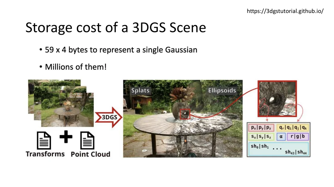
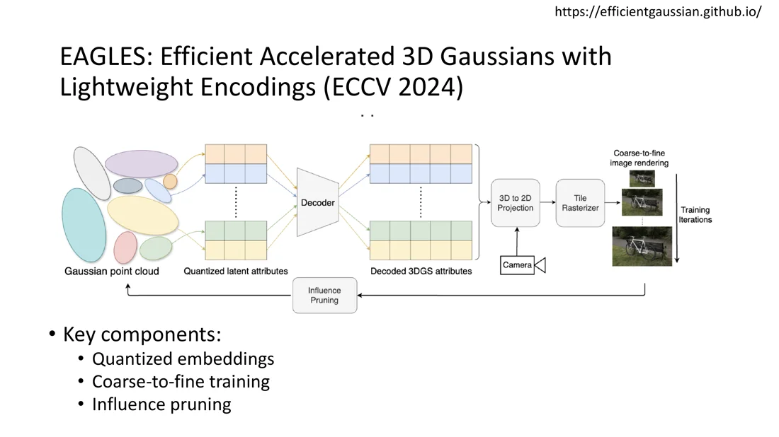
Follow-up works on compression: Compact3D (vector quantization), EAGLES (ECCV 2024), LightGaussian (NeurIPS 2024, 15x reduction, 200+ FPS), Compact 3D Gaussian Representation (CVPR 2024), Compressed 3DGS (CVPR 2024), Reducing the Memory Footprint of 3DGS (I3D 2024).

EAGLES: Efficient Accelerated 3D Gaussians with Lightweight Encodings (ECCV 2024). Key components:

• quantized embeddings: the Gaussian attributes are stored as quantized latents and decoded by a learned decoder, then projected and rasterized
• coarse-to-fine training
• influence pruning: remove Gaussians that contribute little

Slide 37: EAGLES.

Slide 38: 36 MB instead of 357 MB

Slide 38: 81 MB instead of 768 MB

Dynamic Scenes: Dynamic 3D Gaussians

Slides 39-42

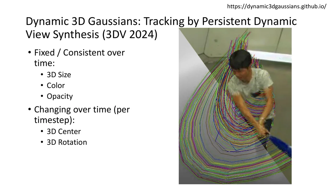
Dynamic 3D Gaussians: Tracking by Persistent Dynamic View Synthesis (3DV 2024). The same Gaussians persist over time:

• fixed / consistent over time: 3D size, color, opacity
• changing per timestep: 3D center, 3D rotation

Because every Gaussian keeps its identity, following its center over time gives dense 3D tracks for free.

Slide 41: Dynamic 3D Gaussians

Slide 42: tracking 3D Gaussians over time

Surface Reconstruction: SuGaR

Slides 43-47

Mesh extraction: the naive way to get a mesh from Gaussian splatting is to run TSDF fusion or marching cubes. Problem: the reconstructed surfaces are not smooth, so the extracted meshes are very noisy (the scene is a fog of overlapping, semi-transparent Gaussians).

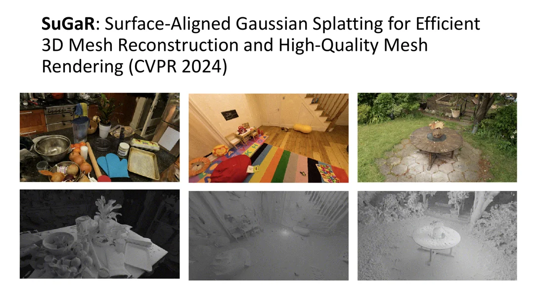
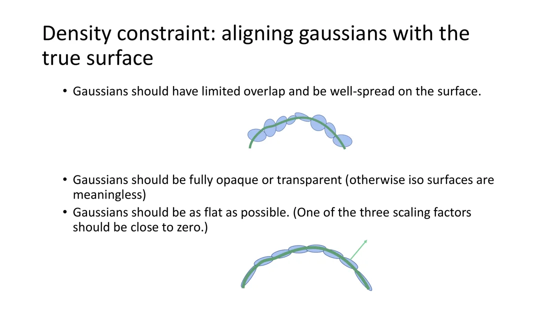
SuGaR: Surface-Aligned Gaussian Splatting for Efficient 3D Mesh Reconstruction and High-Quality Mesh Rendering (CVPR 2024). A density constraint aligns the Gaussians with the true surface:

• Gaussians should have limited overlap and be well spread on the surface.
• Gaussians should be fully opaque or fully transparent (otherwise iso-surfaces are meaningless).
• Gaussians should be as flat as possible: one of the three scaling factors should be close to zero.

Slide 46: SuGaR

Slide 47: aligning Gaussians with the surface

Summary

	NeRF	3D Gaussian Splatting
Representation	implicit, an MLP	explicit, millions of 3D Gaussians, no network
Parameters	network weights	per Gaussian: $\mu$, $R$ (quaternion), $S$, $o$, SH color (59 floats)
$\alpha$	$1-\exp (-{\sigma }_i{\delta }_i)$, computed	$o_i{G}_i^{2D}(\mathbf{x})$, learned opacity × projected Gaussian
Rendering	ray marching, many MLP queries	rasterization: project, global sort, tiles, blend
Speed	slow training, not real time	fast training, 100+ FPS
Initialization	none (random weights)	SfM points
Weaknesses	speed, editing	storage, static scenes, no clean surface

Self-Test

Why is NeRF slow, and how does 3DGS avoid it?

Answer

NeRF queries an MLP for every sample on every ray. 3DGS stores explicit Gaussians and rasterizes them: project, sort, blend. No network at all.

Which parameters does a 3D Gaussian have?

Answer $\mu$, covariance $\Sigma$ (from rotation quaternion and 3 scales), opacity $o$ (sigmoid), color as RGB or spherical harmonics coefficients.

Mean

Why is $\Sigma$ factorized as $RS{S}^T{R}^T$?

Answer $RS{S}^T{R}^T$ with a quaternion rotation and a diagonal scale is always a valid ellipsoid.

A covariance must be positive semi-definite; optimizing its 9 entries directly with gradient descent can make it invalid.

How is a 3D Gaussian projected to the image?

Answer ${\Sigma }^{\prime }=JW\Sigma W^T{J}^T$, with $W$ the viewing transformation and $J$ the Jacobian of the affine approximation of the projection. The result is a 2D Gaussian $\mathcal{N}({\mu }_{2D},{\Sigma }^{\prime })$.

Write down the 3DGS image formation model and explain every symbol.

Answer $C={\sum }_{i\in \mathcal{N}}{\mathbf{c}}_i{\alpha }_i{\prod }_{j=1}^{i-1}(1-{\alpha }_j)$, ${\alpha }_i=o_i{G}_i^{2D}(\mathbf{x})$. $C$: pixel color; $\mathcal{N}$: depth-sorted Gaussians overlapping the pixel; ${\mathbf{c}}_i$: color; $o_i$: learned opacity; $G_i^{2D}(\mathbf{x})$: projected Gaussian at the pixel; the product: transmittance.

What is the same and what is different between the NeRF and 3DGS rendering equations?

Answer $\sum T_i{\alpha }_i{\mathbf{c}}_i$ with $T_i={\prod }_{j<i}(1-{\alpha }_j)$. Different: NeRF's ${\alpha }_i=1-e^{-{\sigma }_i{\delta }_i}$ from MLP samples along a ray; 3DGS's ${\alpha }_i=o_i{G}_i^{2D}(\mathbf{x})$ from sorted explicit Gaussians. This makes 3DGS real time.

Same: alpha compositing

Why does 3DGS render in real time?

Answer $16\times 16$ tiles, each Gaussian assigned only to the tiles it overlaps, one global depth sort, every tile rendered in parallel.

It is a special case of alpha blending that fits the GPU pipeline:

What is adaptive density control?

Answer

The SfM initialization is sparse. During training, Gaussians in under-reconstructed regions are cloned, and oversized Gaussians in over-reconstructed regions are split.

What loss is used?

Answer $\mathcal{L}=(1-\lambda ){\mathcal{L}}_1+\lambda {\mathcal{L}}_{\text{D-SSIM}}$ between rendered and ground-truth images.

Name the three limitations of 3DGS and a follow-up for each.

Answer

High storage (59 floats per Gaussian, millions of them) → compression, e.g. EAGLES (quantized embeddings, coarse-to-fine, pruning). Static scenes → Dynamic 3D Gaussians (only center and rotation change over time, giving 3D tracks). No clean surface → SuGaR (limited overlap, opaque or transparent, flat Gaussians).

Related

• Previous: Lecture 7: NeRF · Next: Lecture 9: Learning-Based 3D Reconstruction · Course: Overview
• Concepts: Gaussian Splatting, Volume Rendering, Quaternion, Structure from Motion, Implicit and Explicit Representations, Point Cloud
• Learning-based reconstruction (DUSt3R, Lecture 9) follows, including 3DGS from few views; 3D Gaussians come back as an output representation of generative models (Lecture 10-11).