Lecture 10: Diffusion Models

TL;DR

1. Single-view reconstruction is ill-posed: a deterministic model collapses to the average. We should learn a distribution of all plausible configurations → generative models.
2. Four families: GANs (adversarial), VAEs (variational lower bound), flows (invertible transform), diffusion (gradually add Gaussian noise, learn to reverse). Trilemma: quality, diversity, speed; diffusion has quality + diversity but is slow.
3. Forward process: $q({\mathbf{x}}_t\mid {\mathbf{x}}_{t-1})=\mathcal{N}(\sqrt{1-{\beta }_t}{\mathbf{x}}_{t-1},{\beta }_t\mathbf{I})$, in closed form ${\mathbf{x}}_t=\sqrt{{\bar{\alpha }}_t}{\mathbf{x}}_0+\sqrt{1-{\bar{\alpha }}_t}\mathbf{ϵ}$. Nothing is learned.
4. Reverse process: a network learns $p_{\theta }({\mathbf{x}}_{t-1}\mid {\mathbf{x}}_t)$. Maximum likelihood is infeasible → negative ELBO → DDPM: predict the noise, $L_{simple}=\Vert \mathbf{ϵ}-{\mathbf{ϵ}}_{\theta }(\sqrt{{\bar{\alpha }}_t}{\mathbf{x}}_0+\sqrt{1-{\bar{\alpha }}_t}\mathbf{ϵ},t){\Vert }^2$.
5. Sampling needs ~1000 steps. DDIM sketches ${\hat{\mathbf{x}}}_0$ and refines (non-Markovian, far fewer steps). Stable Diffusion runs diffusion in a latent space.
6. For 3D: Zero-1-to-3 generates novel views conditioned on $(R,T)$, but views are 3D-inconsistent. Gen-3Diffusion adds an explicit 3DGS at every step. MVGBench evaluates consistency instead of comparison to one ground truth.

Exam relevance

Hint from a fellow student: “Diffusion: slide 35, slide 33, lecture 10: be able to reconstruct the algorithm, be able to reason about the equations. Remember them!” Also: contrast flow matching vs. diffusion (Lecture 11), and “put together pieces, with diffusion to reconstruct depth and the back part of a scene”. See DDPM: Predict the Noise and Training and Sampling Algorithms.

Motivation for Generative Models

Slides 2-11

So far we reconstructed scenes and objects from multiple images (SfM, multi-view stereo, NeRF, Gaussian splatting); NeRF and 3DGS overfit to a set of training images. But tasks like single-view reconstruction are ill-posed: we can’t see what is behind the object.

• A deterministic model might collapse to an average value.
• We should learn a distribution of all possible configurations instead of simply regressing or fitting to observations.

Generating content is a very powerful capability with many applications:

Slide 7: text to 3D object (TRELLIS, Xiang et al., CVPR 2025)

Slide 8: image to 3D object (TRELLIS)

• Image to 3D: a full 3D object from a single image. Still minor artifacts (e.g. the robot’s arms disconnected from the body), but huge progress within a year.
• 3D scenes: SynCity (Engstler et al., CVPR 2025) generates a scene tile by tile; it can’t generate buildings larger than one tile, because tiles are not coordinated.
• 3D worlds: Lyra 2.0 (Nvidia), HY-World 2.0 (Tencent Hunyuan).
• Motion generation: motion sequences from text (UniMotion, Li et al., 3DV 2025).

Slide 9: SynCity

Slide 11: motion generation (UniMotion)

Generative Models: Main Architectures

Slides 12-16

Slide 12: the four main families of generative models.

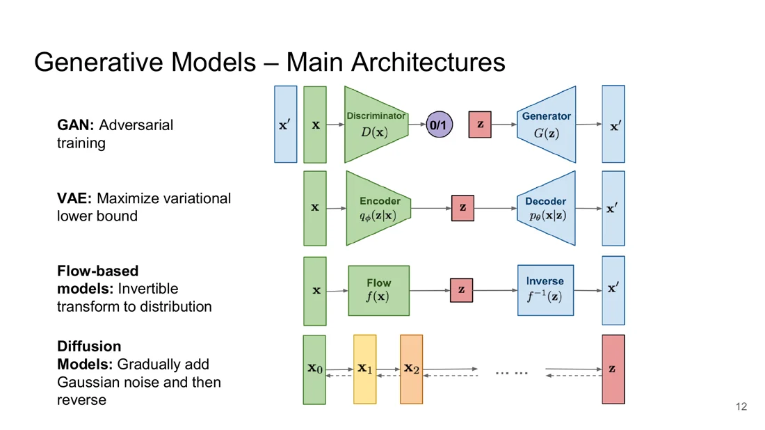
Family	Principle
GAN	adversarial training
VAE	maximize a variational lower bound
Flow-based models	invertible transform to a simple distribution
Diffusion models	gradually add Gaussian noise, then reverse

GAN: a generator $G$ turns random noise into samples that should look like the training data; a discriminator $D$ tries to tell real from generated samples. Training is a min-max game: $G$ tries to fool $D$, $D$ tries to classify correctly. Goal: $G$‘s samples become so realistic that $D$ can’t tell the difference.

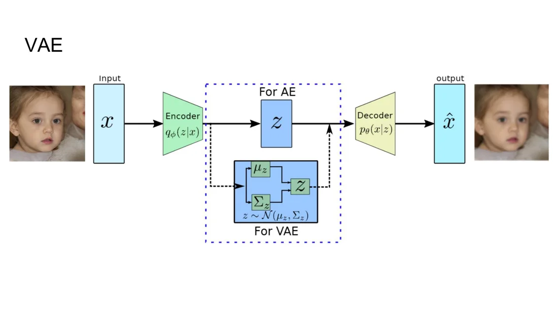
VAE: an autoencoder whose encoder outputs the parameters of a Gaussian in latent space, a mean $\mu$ and a standard deviation $\sigma$. With the reparameterization trick $\mathbf{z}=\mu +\sigma \odot \mathbf{ϵ}$, $\mathbf{ϵ}\sim \mathcal{N}(0,\mathbf{I})$, we can backpropagate through the sampling. The decoder reconstructs the input. Loss = reconstruction loss + KL divergence (keep the latent close to a standard Gaussian).

Diffusion: a forward process $q({\mathbf{x}}_t\mid {\mathbf{x}}_{t-1})$ adds Gaussian noise step by step until the sample is pure noise; a reverse process $p_{\theta }({\mathbf{x}}_{t-1}\mid {\mathbf{x}}_t)$ is trained to remove it step by step.

Slide 14: VAE.

The generative modeling trilemma

	High-quality samples	Mode coverage / diversity	Fast sampling
GANs	✓	✗ (mode collapse)	✓
VAEs, normalizing flows	✗	✓	✓
Denoising diffusion models	✓	✓	✗ (many iterative steps)

Diffusion Models

Idea

Slides 17-23

Diffusion models bridge two distributions: a simple Gaussian (random noisy images) and the complex data distribution (e.g. images of sports balls, which differ in shape, texture, size).

One direction is easy. Which one, and why?

Answer forward process. Nothing is learned; if we keep adding noise, any image converges to noise.

From data to noise: just add noise. Doing this incrementally is the

The idea of diffusion models is to learn the backward process, the incremental denoising: a network takes the current noisy image and tells us how to denoise it. The same network is applied over many steps until we end up with an image of a volleyball.

Slide 19: forward process (data → noise)

Slide 20: learn to undo the noising

Diffusion models are the state of the art for image generation (Stable Diffusion, Flux, Midjourney, DALL-E) and image editing (Flux.1 Kontext: remove objects, change scenes, keep quality). Flow-based models are emerging, but their core architecture is often still diffusion-like.

Diffusion: Theory

Diffusion Probabilistic Models

Slide 25

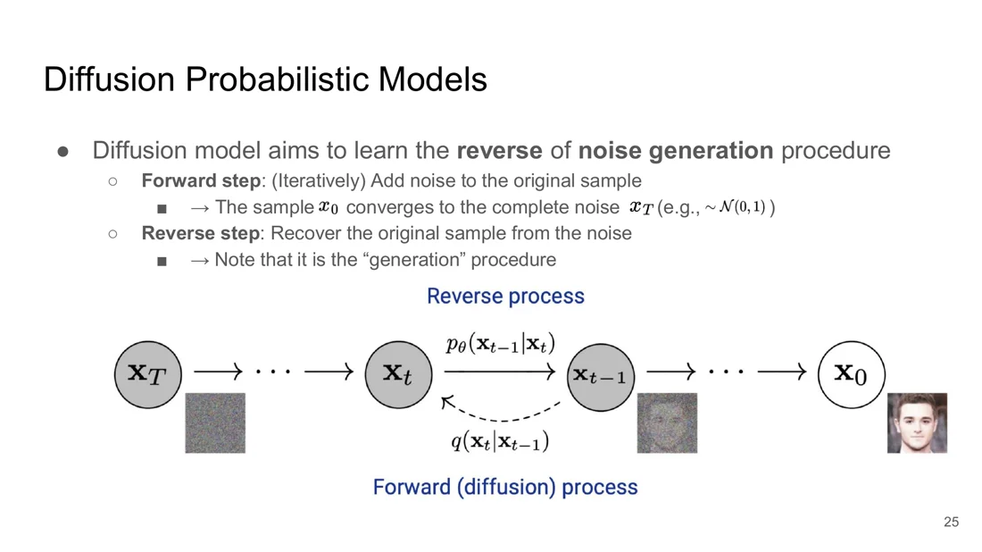
A diffusion model learns the reverse of a noise generation procedure:

• Forward step: iteratively add noise to the original sample ${\mathbf{x}}_0$ → it converges to complete noise ${\mathbf{x}}_T$ (e.g. $\sim \mathcal{N}(0,\mathbf{I})$).
• Reverse step: recover the original sample from the noise → this is the generation procedure.

Slide 25: reverse process p_θ(x_t−1 | x_t) and forward process q(x_t | x_t−1).

Forward Step

Slides 26-28

The forward process is a Markov chain, a product of conditional Gaussians:

Forward process

$$q({\mathbf{x}}_{1:T}\mid {\mathbf{x}}_0)=\prod _{t=1}^{T}q({\mathbf{x}}_t\mid {\mathbf{x}}_{t-1}),q({\mathbf{x}}_t\mid {\mathbf{x}}_{t-1}):=\mathcal{N}({\mathbf{x}}_t;\sqrt{1-{\beta }_t}{\mathbf{x}}_{t-1},{\beta }_t\mathbf{I})$$

Put differently:

$${\mathbf{x}}_t=\sqrt{1-{\beta }_t}{\mathbf{x}}_{t-1}+\sqrt{{\beta }_t}\mathbf{ϵ},\mathbf{ϵ}\sim \mathcal{N}(0,\mathbf{I})$$

${\beta }_t$: the noise schedule (variances), usually fixed beforehand and increased over time. $\sqrt{1-{\beta }_t}$: the variance-preserving factor (it keeps the total variance bounded).

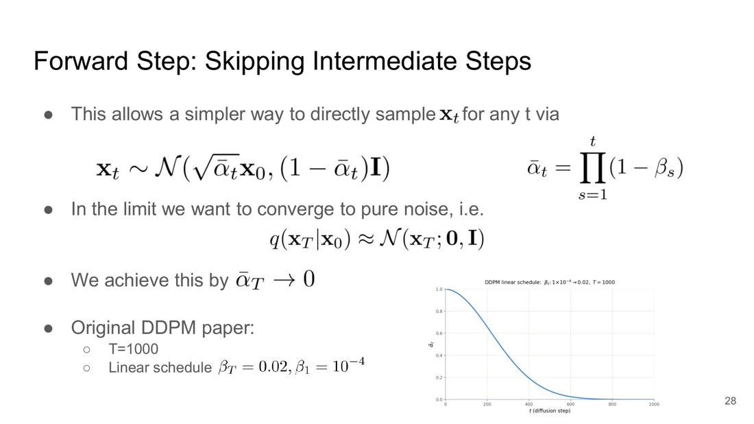
Skipping intermediate steps: the noising doesn’t have to be done step by step. There is a closed form for ${\mathbf{x}}_t$ given ${\mathbf{x}}_0$:

Closed-form forward step

$${\mathbf{x}}_t\sim \mathcal{N}(\sqrt{{\bar{\alpha }}_t}{\mathbf{x}}_0,(1-{\bar{\alpha }}_t)\mathbf{I}),{\bar{\alpha }}_t=\prod _{s=1}^t(1-{\beta }_s)$$

Equivalently ${\mathbf{x}}_t=\sqrt{{\bar{\alpha }}_t}{\mathbf{x}}_0+\sqrt{1-{\bar{\alpha }}_t}\mathbf{ϵ}$.

Why the closed form holds

With ${\alpha }_t=1-{\beta }_t$: ${\mathbf{x}}_t=\sqrt{{\alpha }_t}{\mathbf{x}}_{t-1}+\sqrt{1-{\alpha }_t}{\mathbf{ϵ}}_t$ and ${\mathbf{x}}_{t-1}=\sqrt{{\alpha }_{t-1}}{\mathbf{x}}_{t-2}+\sqrt{1-{\alpha }_{t-1}}{\mathbf{ϵ}}_{t-1}$. Substituting gives $\sqrt{{\alpha }_t{\alpha }_{t-1}}{\mathbf{x}}_{t-2}$ plus two independent Gaussian noises with variances ${\alpha }_t(1-{\alpha }_{t-1})$ and $1-{\alpha }_t$. Their sum is Gaussian with variance $1-{\alpha }_t{\alpha }_{t-1}$. Repeating down to ${\mathbf{x}}_0$ gives $\sqrt{{\bar{\alpha }}_t}{\mathbf{x}}_0+\sqrt{1-{\bar{\alpha }}_t}\mathbf{ϵ}$.

In the limit we want pure noise, $q({\mathbf{x}}_T\mid {\mathbf{x}}_0)\approx \mathcal{N}({\mathbf{x}}_T;0,\mathbf{I})$. We achieve this by ${\bar{\alpha }}_T\to 0$. Original DDPM paper: $T=1000$, linear schedule from ${\beta }_1=10^{-4}$ to ${\beta }_T=0.02$.

Slide 28: ᾱ_t decays to 0 over the steps.

Why not simply choose ${\beta }_t=1$?

Answer ${\bar{\alpha }}_t=0$ immediately, and the first step would throw away all information of the image. Such a step is impossible to undo. We keep ${\beta }_t$ small in the first steps (while the image still carries information) and can afford more noise per step later.

Then

Backward Step / Sampling

Slides 29-30

By design $q({\mathbf{x}}_T\mid {\mathbf{x}}_0)\approx \mathcal{N}(0,\mathbf{I})$. In theory we can generate samples:

1. sample initial random noise ${\mathbf{x}}_T\sim \mathcal{N}(0,\mathbf{I})$
2. iteratively denoise ${\mathbf{x}}_{t-1}\sim q({\mathbf{x}}_{t-1}\mid {\mathbf{x}}_t)$, the unknown true denoising distribution

If ${\beta }_t$ is small, we can approximate $q({\mathbf{x}}_{t-1}\mid {\mathbf{x}}_t)$ with a Gaussian, whose mean is a trainable network:

Reverse process

$$p_{\theta }({\mathbf{x}}_{t-1}\mid {\mathbf{x}}_t)=\mathcal{N}({\mathbf{x}}_{t-1};{\mathbf{\mu }}_{\theta }({\mathbf{x}}_t,t),{\sigma }_t^2\mathbf{I}),p_{\theta }({\mathbf{x}}_{0:T})=p({\mathbf{x}}_T)\prod _{t=1}^T{p}_{\theta }({\mathbf{x}}_{t-1}\mid {\mathbf{x}}_t),p({\mathbf{x}}_T)=\mathcal{N}({\mathbf{x}}_T;0,\mathbf{I})$$

Goal: maximum likelihood ${\max }_{\theta }{\mathbb{E}}_{q({\mathbf{x}}_0)}[\log p_{\theta }({\mathbf{x}}_0)]$. This needs marginalizing over all possible paths ending in ${\mathbf{x}}_0$, $p_{\theta }({\mathbf{x}}_0)=\int p_{\theta }({\mathbf{x}}_{0:T})d{\mathbf{x}}_{1:T}$. Infeasible!

Derivation of the Diffusion Loss

Slides 31-32

With Jensen’s inequality we get a negative ELBO (an upper bound on the negative log-likelihood, which we minimize):

$${\mathbb{E}}_q[-\log p_{\theta }({\mathbf{x}}_0)]\le {\mathbb{E}}_q\left[-\log \frac{p_{\theta }({\mathbf{x}}_{0:T})}{q({\mathbf{x}}_{1:T}\mid {\mathbf{x}}_0)}\right]$$

which can be rewritten as three terms:

Decomposition of the ELBO

$${\mathbb{E}}_q[\underset{L_T}{\underbrace{D_{KL}(q({\mathbf{x}}_T\mid {\mathbf{x}}_0)\Vert p({\mathbf{x}}_T))}}+\sum _{t>1}\underset{L_{t-1}}{\underbrace{D_{KL}(q({\mathbf{x}}_{t-1}\mid {\mathbf{x}}_t,{\mathbf{x}}_0)\Vert p_{\theta }({\mathbf{x}}_{t-1}\mid {\mathbf{x}}_t))}}\underset{L_0}{\underbrace{-\log p_{\theta }({\mathbf{x}}_0\mid {\mathbf{x}}_1)}}]$$

1. $L_T$ prior matching: independent of $\theta$ (no learnable parameters) → constant, dropped.
2. $L_{t-1}$ denoising matching: match the true denoising distribution (conditioned on ${\mathbf{x}}_0$, which is tractable) with the learned one.
3. $L_0$ reconstruction term: scores the model against an actual data value.

(The derivation of the three terms is skipped in the lecture.) Because everything is Gaussian, all these KL terms reduce to simple L2 losses.

DDPM: Predict the Noise

Slides 33-34

Key idea of DDPM (Ho et al., 2020)

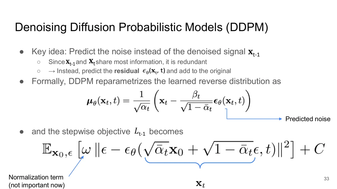
Predict the noise instead of the denoised signal. ${\mathbf{x}}_{t-1}$ and ${\mathbf{x}}_t$ share most of their information, so predicting it again is redundant. Instead, predict the residual ${\mathbf{ϵ}}_{\theta }({\mathbf{x}}_t,t)$ and remove it.

DDPM reparameterization (Slide 33)

$${\mathbf{\mu }}_{\theta }({\mathbf{x}}_t,t)=\frac{1}{\sqrt{{\alpha }_t}}\left({\mathbf{x}}_t-\frac{{\beta }_t}{\sqrt{1-{\bar{\alpha }}_t}}{\mathbf{ϵ}}_{\theta }({\mathbf{x}}_t,t)\right)$$

and the stepwise objective $L_{t-1}$ becomes

$${\mathbb{E}}_{{\mathbf{x}}_0,\mathbf{ϵ}}[\omega \Vert \mathbf{ϵ}-{\mathbf{ϵ}}_{\theta }(\underset{{\mathbf{x}}_t}{\underbrace{\sqrt{{\bar{\alpha }}_t}{\mathbf{x}}_0+\sqrt{1-{\bar{\alpha }}_t}\mathbf{ϵ}}},t\left){\Vert }^2\right]+C$$

${\mathbf{ϵ}}_{\theta }$: the predicted noise; $\omega$: a normalization (weighting) term; $C$: a constant.

Symbol	Meaning
${\mathbf{x}}_0$	clean data sample
${\mathbf{x}}_t$	noisy sample at step $t$
$\mathbf{ϵ}\sim \mathcal{N}(0,\mathbf{I})$	the true noise added in the forward process
${\mathbf{ϵ}}_{\theta }({\mathbf{x}}_t,t)$	the network’s prediction of that noise
${\beta }_t$	noise schedule; ${\alpha }_t=1-{\beta }_t$
${\bar{\alpha }}_t={\prod }_{s\le t}{\alpha }_s$	how much of ${\mathbf{x}}_0$ is left at step $t$
${\sigma }_t$	standard deviation of the fresh noise in the reverse step

Slide 33: DDPM.

Simplified training objective (Slide 34)

Ho et al. drop the weights and sample $t$ at random:

$$L_{simple}(\theta ):={\mathbb{E}}_{t,{\mathbf{x}}_0,\mathbf{ϵ}}[\Vert \mathbf{ϵ}-{\mathbf{ϵ}}_{\theta }(\sqrt{{\bar{\alpha }}_t}{\mathbf{x}}_0+\sqrt{1-{\bar{\alpha }}_t}\mathbf{ϵ},t\left){\Vert }^2\right],t\sim \mathcal{U}(1,T),{\mathbf{x}}_0\sim q({\mathbf{x}}_0),\mathbf{ϵ}\sim \mathcal{N}(0,\mathbf{I})$$

The reconstruction term $L_0=-\log p_{\theta }({\mathbf{x}}_0\mid {\mathbf{x}}_1)$ is approximately included ($t=1$).

Why the mean formula makes sense

From the closed form, ${\mathbf{x}}_0=\frac{1}{\sqrt{{\bar{\alpha }}_t}}({\mathbf{x}}_t-\sqrt{1-{\bar{\alpha }}_t}\mathbf{ϵ})$: knowing the noise means knowing the clean image. The reverse mean removes the fraction $\frac{{\beta }_t}{\sqrt{1-{\bar{\alpha }}_t}}$ of the predicted noise that was added in the last step, and rescales by $\frac{1}{\sqrt{{\alpha }_t}}$ to undo the variance-preserving shrinking $\sqrt{1-{\beta }_t}$.

Training and Sampling Algorithms

Slide 35

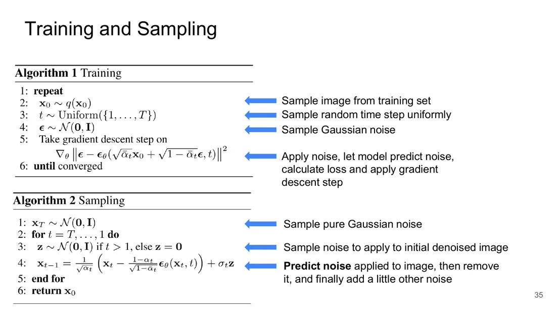
Algorithm 1: Training

1. repeat
2. ${\mathbf{x}}_0\sim q({\mathbf{x}}_0)$: sample an image from the training set
3. $t\sim \text{Uniform}(\{1,\dots ,T\})$: sample a random time step uniformly
4. $\mathbf{ϵ}\sim \mathcal{N}(0,\mathbf{I})$: sample Gaussian noise
5. take a gradient descent step on ${\nabla }_{\theta }\Vert \mathbf{ϵ}-{\mathbf{ϵ}}_{\theta }(\sqrt{{\bar{\alpha }}_t}{\mathbf{x}}_0+\sqrt{1-{\bar{\alpha }}_t}\mathbf{ϵ},t){\Vert }^2$: apply noise, let the model predict it, compute the loss, update
6. until converged

Algorithm 2: Sampling

1. ${\mathbf{x}}_T\sim \mathcal{N}(0,\mathbf{I})$: sample pure Gaussian noise
2. for $t=T,\dots ,1$ do
3. $\mathbf{z}\sim \mathcal{N}(0,\mathbf{I})$ if $t>1$, else $\mathbf{z}=0$: sample noise to re-inject
4. ${\mathbf{x}}_{t-1}=\frac{1}{\sqrt{{\alpha }_t}}\left({\mathbf{x}}_t-\frac{1-{\alpha }_t}{\sqrt{1-{\bar{\alpha }}_t}}{\mathbf{ϵ}}_{\theta }({\mathbf{x}}_t,t)\right)+{\sigma }_t\mathbf{z}$: predict the noise, remove it, add a little fresh noise
5. end for
6. return ${\mathbf{x}}_0$

Slide 35: training and sampling.

Typical mistakes

• Training does not run the chain step by step: it jumps to a random $t$ with the closed form.
• The network predicts the noise $\mathbf{ϵ}$, not ${\mathbf{x}}_{t-1}$ or ${\mathbf{x}}_0$.
• In sampling, $1-{\alpha }_t={\beta }_t$ (same as in the mean formula of Slide 33).
• The last step ($t=1$) adds no noise ($\mathbf{z}=0$).

flowchart LR
  subgraph TR["Training (one step)"]
    direction LR
    A["x₀ from data"] --> B["t ~ U(1..T), ε ~ N(0,I)"] --> C["x_t = √ᾱ_t x₀ + √(1−ᾱ_t) ε"] --> D["ε_θ(x_t, t)"] --> E["‖ε − ε_θ‖² → gradient step"]
  end
  subgraph SA["Sampling"]
    direction LR
    F["x_T ~ N(0,I)"] --> G["for t = T..1:<br/>x_{t−1} = 1/√α_t (x_t − β_t/√(1−ᾱ_t) ε_θ) + σ_t z"] --> H["x₀"]
  end

Sampling is slow: it often requires 1000 reverse steps.

Slide 37: less noise at the start → less diversity in the samples.

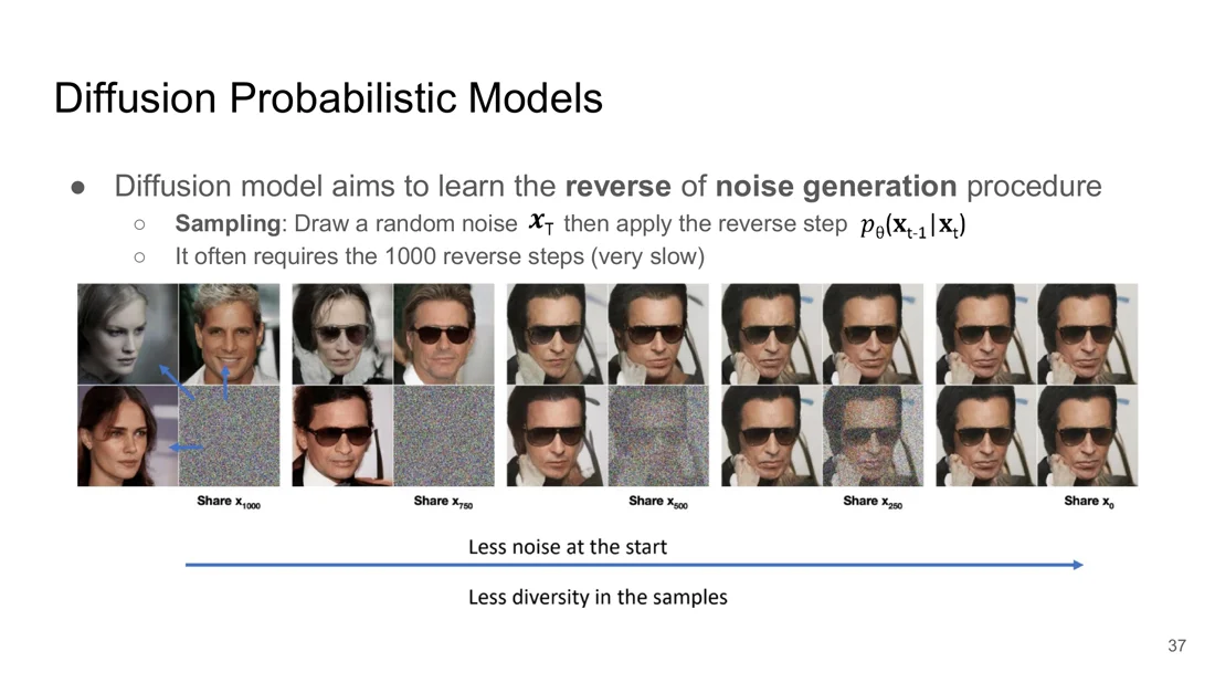
What happens if we don't start from pure noise, but from a partially noised image?

Answer

The less noise at the start, the closer the generated images are to each other (less diversity). With no noise at all, the output is always the same (deterministic). Pure noise gives the most diverse outputs. This is also how diffusion-based image editing works.

DDIM: Faster Sampling

Slides 38-41

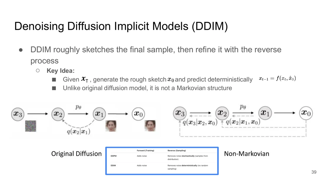
Motivation: diffusion is slow because of the iterative procedure; GANs and VAEs create a sample in one forward pass. Can we combine the advantages? Instead of naively applying diffusion on top of a GAN/VAE, DDIM (Denoising Diffusion Implicit Models) proposes a principled rough sketch + refinement:

• given ${\mathbf{x}}_T$, generate a rough sketch ${\hat{\mathbf{x}}}_0$ and predict deterministically ${\mathbf{x}}_{t-1}=f({\mathbf{x}}_t,{\hat{\mathbf{x}}}_0)$
• unlike the original diffusion model, it is not Markovian: the reverse step depends on ${\hat{\mathbf{x}}}_0$

Slide 39: original (Markovian) diffusion vs. DDIM (non-Markovian).

DDIM

Forward process (same marginals as DDPM; here ${\alpha }_t$ denotes the cumulative product):

$${\mathbf{x}}_t=\sqrt{{\alpha }_t}{\mathbf{x}}_0+\sqrt{1-{\alpha }_t}\mathbf{ϵ},\mathbf{ϵ}\sim \mathcal{N}(0,\mathbf{I})$$

Reverse process:

$${\mathbf{x}}_{t-1}=\sqrt{{\alpha }_{t-1}}\underset{\text{"predicted }{\mathbf{x}}_0\text{"}}{\underbrace{\left(\frac{{\mathbf{x}}_t-\sqrt{1-{\alpha }_t}{\mathbf{ϵ}}_{\theta }^{(t)}({\mathbf{x}}_t)}{\sqrt{{\alpha }_t}}\right)}}+\underset{\text{"direction pointing to }{\mathbf{x}}_t\text{"}}{\underbrace{\sqrt{1-{\alpha }_{t-1}-{\sigma }_t^2}\cdot {\mathbf{ϵ}}_{\theta }^{(t)}({\mathbf{x}}_t)}}+\underset{\text{random noise}}{\underbrace{{\sigma }_t{\mathbf{ϵ}}_t}}$$

With ${\sigma }_t=0$ the sampling is fully deterministic.

Notation

On the DDIM slides, ${\alpha }_t$ is what the DDPM slides call ${\bar{\alpha }}_t$ (the cumulative product).

DDIM significantly reduces the number of sampling steps: it creates the outline of the sample after only 100 steps (DDPM needs thousands), even usable results with 10.

Stable Diffusion: Diffusion in Latent Space

Slides 42-44

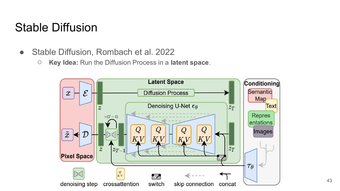
Problem with standard diffusion: DDPM operates directly on images, which are high-dimensional (a $512\times 512$ RGB image has 786,432 values). This makes it slow to train, expensive to sample and memory-intensive.

Stable Diffusion (Rombach et al., 2022). Key idea: run the diffusion process in a latent space.

• An encoder $\mathcal{E}$ maps the image $x$ into a compact latent $z$; the forward and reverse diffusion run on $z$; a decoder $\mathcal{D}$ maps the denoised latent back to pixels.
• The denoising U-Net ${ϵ}_{\theta }$ uses self-attention (understand the image globally) and cross-attention to condition on text, semantic maps, images or other representations via an encoder ${\tau }_{\theta }$.
• Large-scale training: LAION-5B, 5 billion images with text annotations.

Slide 43: Stable Diffusion (latent diffusion).

Multi-View Image Diffusion for 3D

Slides 45-46

Do 2D diffusion models have knowledge about the 3D domain? How can we leverage image diffusion for 3D?

Multi-view diffusion: produce multiple views of the same object or scene that are geometrically consistent (e.g. down 30°, left 90°).

Zero-1-to-3

Slides 47-52

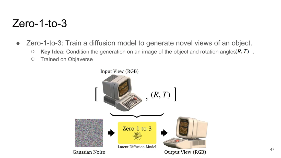
Zero-1-to-3: train a diffusion model to generate novel views of an object. Built on Stable Diffusion, trained on Objaverse. Key idea: condition the generation on an image of the object and the relative rotation and translation $(R,T)$.

Zero-1-to-3 training objective

$$\underset{\theta }{\min }{\mathbb{E}}_{z\sim \mathcal{E}(x),t,\mathbf{ϵ}\sim \mathcal{N}(0,1)}\Vert \mathbf{ϵ}-{\mathbf{ϵ}}_{\theta }(z_t,t,c(x,R,T)){\Vert }_2^2$$

$c(x,R,T)$: the embedding of the input view and the relative camera extrinsics. The same objective as a latent diffusion model, only with this extra conditioning.

Slide 47: Zero-1-to-3.

Reconstruction: a neural field is optimized so that its renderings match the input view (MSE) and, from other viewpoints $(R_i,T_i)$, are guided by gradients from Zero-1-to-3 (a score-distillation-style loss, $\nabla {\mathcal{L}}_{SJC}$, → Lecture 11).

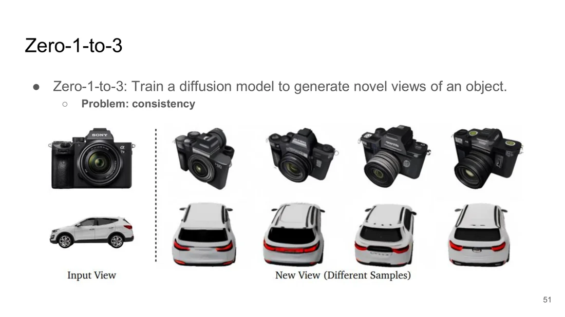
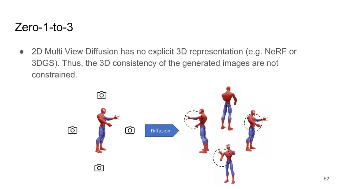
Problem: consistency. Sampling the same new view several times gives different results (different camera lenses, different cars). 2D multi-view diffusion has no explicit 3D representation (like NeRF or 3DGS), so the 3D consistency of the generated images is not constrained: every view is generated independently.

Slide 51: inconsistent samples

Slide 52: no explicit 3D representation

Limitations of Multi-View Diffusion

Slides 53-58

• Generating novel views independently leads to 3D inconsistencies.
• Synchronized denoising with crosstalk (Zero123++, SyncDreamer, …) helps, but cannot ensure accurate consistency (the unicorn looks left in one view, right in another).
• Inconsistent multi-view images lead to implausible 3D reconstructions when fed to a sparse-view reconstructor (NeRF / SDF / 3DGS regressor), e.g. floating 3D Gaussian splats with LGM.

Key questions: How can we get rid of 3D inconsistencies (→ Gen-3Diffusion)? How can we quantify inconsistencies and performance (→ MVGBench)?

Slide 58: add a consistency refinement at every diffusion step.

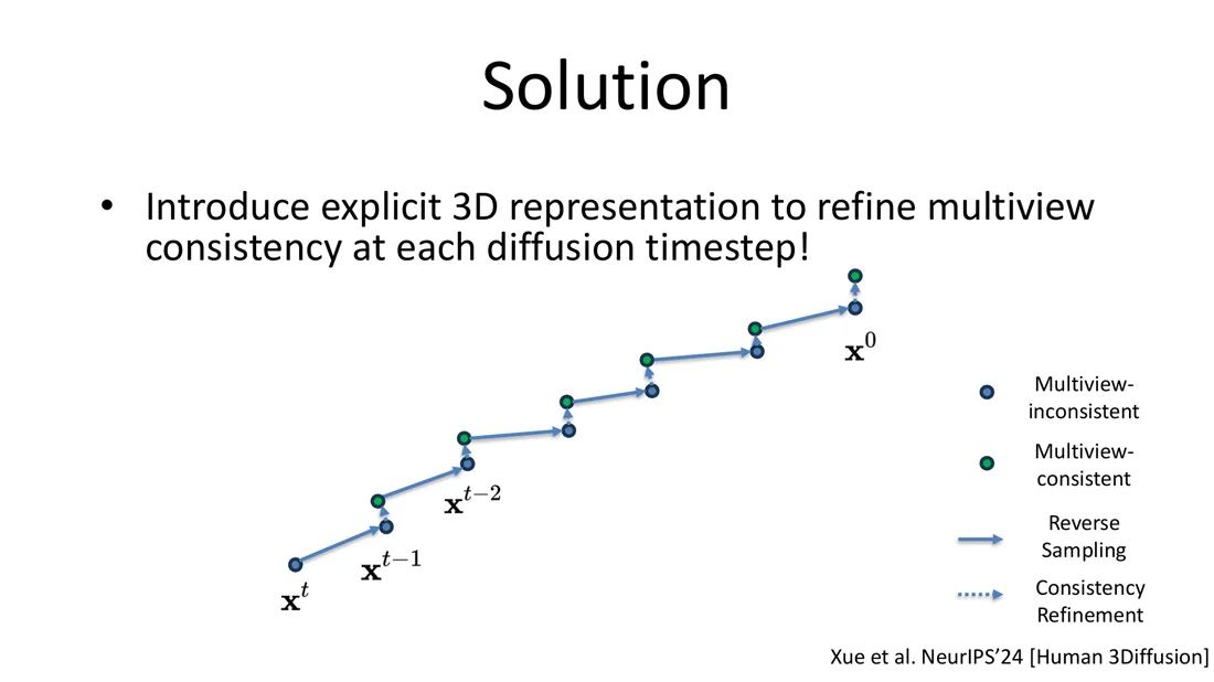
Problem: the multi-view diffusion process lacks an explicit 3D representation, so its trajectory drifts away from the multi-view consistent samples. Solution: introduce an explicit 3D representation to refine multi-view consistency at each diffusion timestep.

Gen-3Diffusion

Slides 59-65

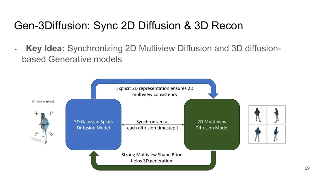
Gen-3Diffusion (Xue et al., NeurIPS 2024 “Human 3Diffusion”, PAMI 2025). Key idea: synchronize a 2D multi-view diffusion model and a 3D diffusion-based generative model (3D Gaussian splats) at every diffusion timestep:

• the explicit 3D representation ensures 2D multi-view consistency
• the strong multi-view shape prior from the 2D model helps the 3D generation

At each step, the 3D model takes the input view and the current noisy multi-view images, generates 3D Gaussians, renders them to consistent multi-view images, and these are used in the next denoising step.

Slide 59: synchronizing 2D multi-view diffusion and 3D reconstruction.

Results: better appearance and geometry than avatar methods (SiTH, SiFU, ICON, ECON) and than novel-view diffusion (Zero123-XL, SV3D). It generalizes strongly (even to multiple people), thanks to the pre-trained 2D diffusion model.

Slide 65: strong generalization (3DGS renderings).

Multi-View Diffusion and Ground Truth: MVGBench

Slides 66-73

Reconstructing an object from a single image is ill-posed, but benchmarks compare against ground-truth data. What is ground truth in a generative task?

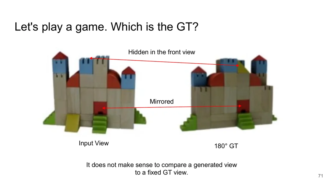
Given the front view of a toy castle, which of the four generated back views is the ground truth?

Answer It does not make sense to compare a generated view to a fixed GT view.

You can’t tell: the back is not visible in the input. The real back even has a yellow triangle hidden in the front view and a mirrored, slightly asymmetric staircase. A plausible, consistent back view should not be penalized just because it differs from one fixed GT.

Slide 69: the true back view contains things hidden in the front view.

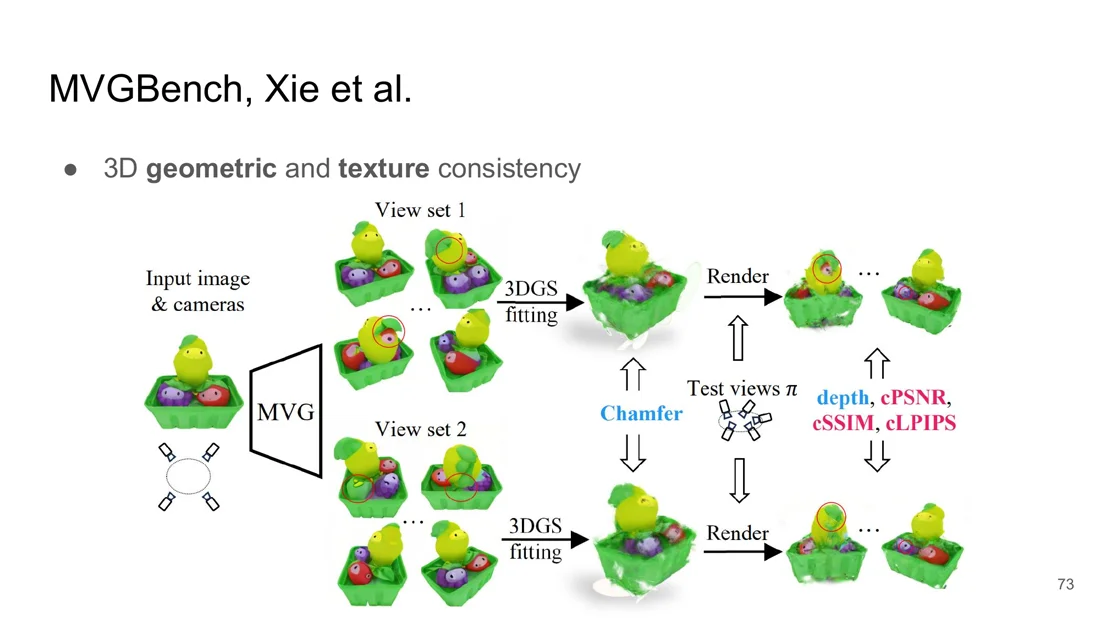
MVGBench (Xie et al., ICCV 2025): a comprehensive benchmark that evaluates

• 3D geometric consistency (Chamfer distance, depth)
• 3D texture consistency (cSSIM, cPSNR, cLPIPS)
• image quality (oFID, IQ-vlm)
• semantic consistency (style, object class, color)

How it works: generate two independent sets of views from the same input, fit a 3DGS to each, and compare the two reconstructions (render test views, compute Chamfer, depth, cPSNR, …). If the generated views are internally consistent, both reconstructions agree.

Slide 71: 3D geometric and texture consistency in MVGBench.

Semantic and quality metrics: FID compares distributions (not one GT image):

$$\text{FID}(r,g)=\Vert {\mu }_r-{\mu }_g{\Vert }_2^2+\text{Tr}\left({\Sigma }_r+{\Sigma }_g-2\sqrt{{\Sigma }_r{\Sigma }_g}\right)$$

($\mu ,\Sigma$: mean and covariance of real and generated features), plus a pre-trained VLM for question answering on quality and for class, color and style consistency.

Finding: there is a trade-off between image quality and 3D consistency. No existing method (Zero123, SV3D, SyncDreamer, …) achieves both.

Conclusion

Slide 74

• How diffusion models work
• How diffusion models can generate multi-view images
• Limitations of multi-view diffusion

Next lecture: other ways to use diffusion for 3D: Score Distillation Sampling; methods that don’t rely on image diffusion: point diffusion, Hunyuan3D 2.0, TRELLIS.

Worked Example: One Forward and One Reverse Step

Numbers for the closed form and the sampling step

Take ${\bar{\alpha }}_t=0.36$ at some step $t$, and a pixel $x_0=1.0$, noise $ϵ=0.5$:

$$x_t=\sqrt{0.36}\cdot 1.0+\sqrt{1-0.36}\cdot 0.5=0.6+0.8\cdot 0.5=1.0$$

If the network predicts the noise perfectly, ${ϵ}_{\theta }=0.5$, the implied clean value is

$${\hat{x}}_0=\frac{x_t-\sqrt{1-{\bar{\alpha }}_t}{ϵ}_{\theta }}{\sqrt{{\bar{\alpha }}_t}}=\frac{1.0-0.4}{0.6}=1.0$$

Training minimizes $(ϵ-{ϵ}_{\theta }{)}^2$; here the loss would be 0. In sampling, the step removes only the part $\frac{{\beta }_t}{\sqrt{1-{\bar{\alpha }}_t}}{ϵ}_{\theta }$ of this noise, rescales by $\frac{1}{\sqrt{{\alpha }_t}}$, and adds ${\sigma }_{t}z$.

Self-Test

Why do we need generative models for single-view reconstruction?

Answer

The task is ill-posed: the back of the object is not visible. A deterministic model collapses to the average; a generative model learns the distribution of plausible configurations and can sample diverse outputs.

Explain the generative trilemma for GANs, VAEs and diffusion models.

Answer

GANs: high quality, fast, but low diversity (mode collapse). VAEs/flows: diverse and fast, but lower quality. Diffusion: high quality and diversity, but slow sampling.

Write down the forward step and its closed form. What must hold for ${\bar{\alpha }}_T$?

Answer $q({\mathbf{x}}_t\mid {\mathbf{x}}_{t-1})=\mathcal{N}(\sqrt{1-{\beta }_t}{\mathbf{x}}_{t-1},{\beta }_t\mathbf{I})$; closed form ${\mathbf{x}}_t=\sqrt{{\bar{\alpha }}_t}{\mathbf{x}}_0+\sqrt{1-{\bar{\alpha }}_t}\mathbf{ϵ}$ with ${\bar{\alpha }}_t={\prod }_{s\le t}(1-{\beta }_s)$. For pure noise at the end, ${\bar{\alpha }}_T\to 0$.

Why can't we train with maximum likelihood directly, and what do we do instead?

Answer $p_{\theta }({\mathbf{x}}_0)$ needs marginalizing over all paths ${\mathbf{x}}_{1:T}$, which is infeasible. Instead we minimize the negative ELBO (Jensen), which decomposes into prior matching $L_T$ (constant, dropped), denoising matching $L_{t-1}$ (KL between Gaussians → L2) and reconstruction $L_0$.

What is the key idea of DDPM, and what is the simplified loss?

Answer ${\mathbf{x}}_t$ and ${\mathbf{x}}_{t-1}$ share most information. ${\mathbf{\mu }}_{\theta }=\frac{1}{\sqrt{{\alpha }_t}}({\mathbf{x}}_t-\frac{{\beta }_t}{\sqrt{1-{\bar{\alpha }}_t}}{\mathbf{ϵ}}_{\theta })$. $L_{simple}={\mathbb{E}}_{t,{\mathbf{x}}_0,\mathbf{ϵ}}\Vert \mathbf{ϵ}-{\mathbf{ϵ}}_{\theta }(\sqrt{{\bar{\alpha }}_t}{\mathbf{x}}_0+\sqrt{1-{\bar{\alpha }}_t}\mathbf{ϵ},t){\Vert }^2$.

Predict the noise instead of the denoised image, since

Reconstruct the DDPM training algorithm.

Answer ${\mathbf{x}}_0\sim q({\mathbf{x}}_0)$; $t\sim \text{Uniform}\{\mathrm{1..}T\}$; $\mathbf{ϵ}\sim \mathcal{N}(0,I)$; gradient step on $\Vert \mathbf{ϵ}-{\mathbf{ϵ}}_{\theta }(\sqrt{{\bar{\alpha }}_t}{\mathbf{x}}_0+\sqrt{1-{\bar{\alpha }}_t}\mathbf{ϵ},t){\Vert }^2$; until converged.

Repeat:

Reconstruct the DDPM sampling algorithm.

Answer ${\mathbf{x}}_T\sim \mathcal{N}(0,I)$. For $t=T..1$: $\mathbf{z}\sim \mathcal{N}(0,I)$ if $t>1$ else $0$; ${\mathbf{x}}_{t-1}=\frac{1}{\sqrt{{\alpha }_t}}({\mathbf{x}}_t-\frac{1-{\alpha }_t}{\sqrt{1-{\bar{\alpha }}_t}}{\mathbf{ϵ}}_{\theta }({\mathbf{x}}_t,t))+{\sigma }_t\mathbf{z}$. Return ${\mathbf{x}}_0$.

How does DDIM speed up sampling?

Answer ${\hat{\mathbf{x}}}_0$ from the predicted noise and moves towards it (non-Markovian): ${\mathbf{x}}_{t-1}=\sqrt{{\alpha }_{t-1}}{\hat{\mathbf{x}}}_0+\sqrt{1-{\alpha }_{t-1}-{\sigma }_t^2}{\mathbf{ϵ}}_{\theta }+{\sigma }_t{\mathbf{ϵ}}_t$; deterministic with ${\sigma }_t=0$. It needs about 100 instead of 1000 steps.

It predicts a rough sketch

What is the key idea of Stable Diffusion?

Answer $\mathcal{E}$, decoder $\mathcal{D}$), with a U-Net that uses cross-attention for conditioning (text, images). Trained on LAION-5B.

Run diffusion in the compact latent space of an autoencoder (encoder

How does Zero-1-to-3 work, and what is its main problem?

Answer $(R,T)$, trained on Objaverse, generates novel views. Views are generated independently without an explicit 3D representation, so they are 3D-inconsistent.

A latent diffusion model conditioned on an input image and the relative camera pose

Why evaluate multi-view generation with MVGBench instead of comparing to ground truth?

Answer

Single-view 3D is ill-posed; many backs are plausible. MVGBench measures self-consistency: two independent view sets → two 3DGS reconstructions → compare them (geometry, texture), plus image quality and semantic metrics.

Related

• Previous: Lecture 9: Learning-Based 3D Reconstruction · Next: Lecture 11: Flow Matching and 3D Generation · Course: Overview
• Concepts: Diffusion Model, Attention, Gaussian Splatting, Depth Ambiguity
• Flow matching, score distillation sampling, point cloud diffusion and TRELLIS follow in Lecture 11.