Lecture 6.2: Point Cloud Processing

TL;DR

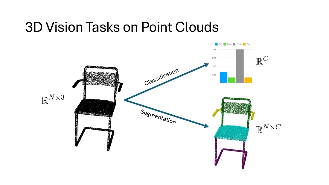
1. Point clouds are unordered sets without connectivity, with uneven density and missing parts. Tasks: classification (${\mathbb{R}}^{N\times 3}\to {\mathbb{R}}^C$) and segmentation (${\mathbb{R}}^{N\times 3}\to {\mathbb{R}}^{N\times C}$).
2. Projection-based (multi-view 2D CNNs) and voxel-based (3D CNNs) approaches lose geometric information. Point-based networks consume the points directly and need permutation invariance, a variable number of points, and locality awareness.
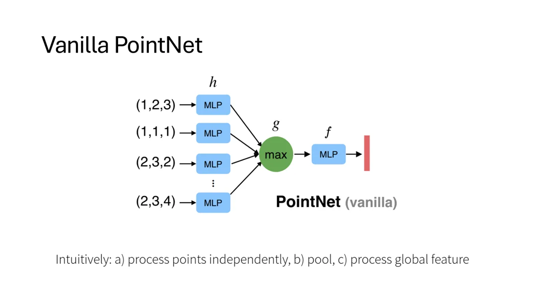
3. PointNet: a shared per-point MLP $h$, a symmetric pooling $g=\max$ and an MLP $f$: $f(g(h({\mathbf{x}}_1),\dots ,h({\mathbf{x}}_n)))$. T-Nets undo rotations; segmentation concatenates local and global features.
4. PointNet++ adds locality: farthest point sampling, grouping neighbors, a PointNet per group, stacked into a hierarchy; feature propagation by interpolation for segmentation.
5. Point Transformer: vector attention over kNN neighborhoods with a relative positional encoding $\delta =\theta ({\mathbf{p}}_i-{\mathbf{p}}_j)$.

flowchart LR
  A["PointNet<br/>permutation invariance"] --> B["PointNet++<br/>locality"] --> C["Point Transformer<br/>vector attention"]

Exam relevance

Block D of the study plan: point-based learning is multiple-choice material (PointNet: why max pooling, permutation invariance; PointNet++: FPS and grouping; scalar vs. vector attention).

Recap: Point Clouds

Slides 2-3

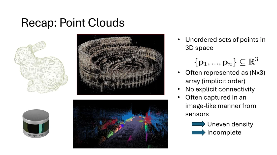
• Unordered sets of points in 3D space: $\{{\mathbf{p}}_1,\dots ,{\mathbf{p}}_n\}\subseteq {\mathbb{R}}^3$
• often represented as an $(N\times 3)$ array (an implicit, meaningless order)
• no explicit connectivity
• often captured in an image-like manner from sensors (LiDAR) → uneven density, incomplete

Slide 2: point clouds

Slide 3: classification and segmentation

Three Families of Approaches

Slides 4-8

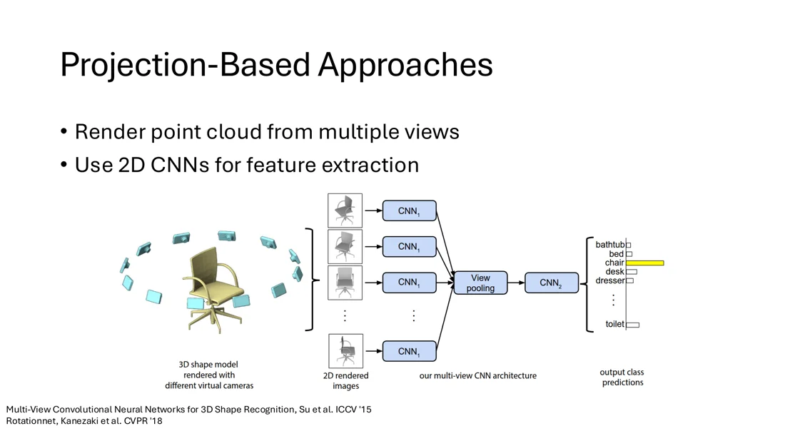
Projection-based: render the point cloud from multiple views, extract features with 2D CNNs, pool over the views and predict the class (Multi-View CNN, Su et al., ICCV 2015; RotationNet, Kanezaki et al., CVPR 2018).

• ✗ geometric information inside the point cloud is collapsed
• ✗ the sparsity of point clouds is under-utilized
• ✗ the choice of views heavily influences the performance

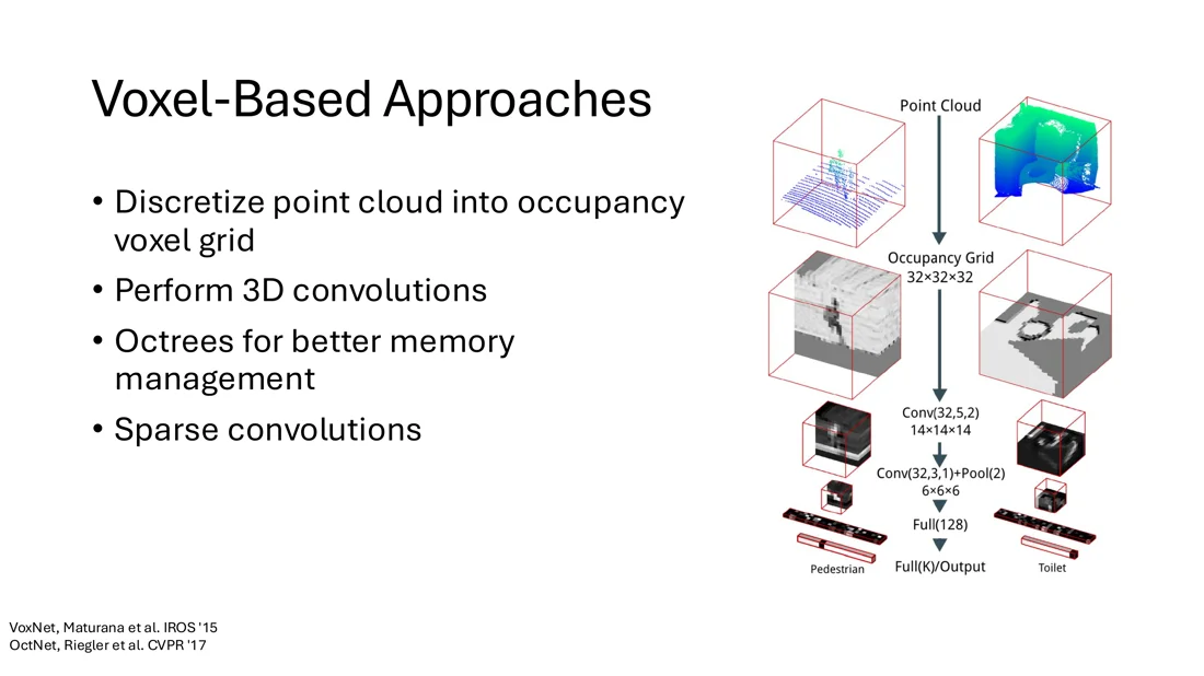
Voxel-based: discretize the point cloud into an occupancy voxel grid and run 3D convolutions (VoxNet, Maturana et al., IROS 2015). Octrees for better memory management (OctNet, Riegler et al., CVPR 2017), sparse convolutions that are only evaluated at occupied voxels.

• ✗ loss of geometric details due to quantization, unless the resolution (and memory) is very high

Slide 4: projection-based

Slide 6: voxel-based

Point-based networks

A network that directly consumes points. Desired properties:

• permutation invariance
• a variable number of points
• locality awareness (reasoning about local neighborhoods)

PointNet

Permutation Invariance

Slides 9-12

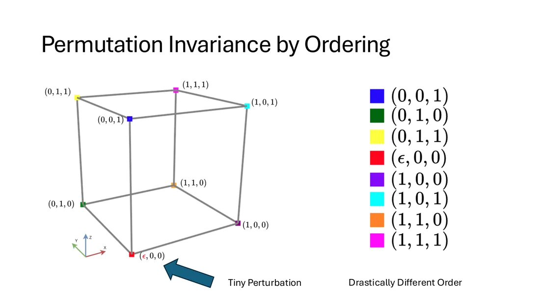
Can we get permutation invariance by sorting the points in a canonical order (e.g. lexicographically by coordinates)?

Answer tiny perturbation (e.g. $(0,0,0)\to (ϵ,0,0)$) can give a drastically different order. In high dimensions there is no ordering that is stable w.r.t. point perturbations. A network on ordered points would be very sensitive to the slightest change.

No. A

Slide 10: a tiny perturbation, a drastically different order.

Symmetric (permutation-invariant) function

$$f({\mathbf{x}}_1,\dots ,{\mathbf{x}}_n)=f({\mathbf{x}}_{\pi (1)},\dots ,{\mathbf{x}}_{\pi (n)})\text{for every permutation }\pi$$

Examples: pooling, $f={\max }_i{\mathbf{x}}_i$ or $f={\text{mean}}_i{\mathbf{x}}_i$ (applied per channel, ${\mathbf{x}}_i\in {\mathbb{R}}^d\to \mathbf{y}\in {\mathbb{R}}^d$). Note: this also allows a variable number of input points.

From Symmetric Functions to PointNet

Slides 13-15

Per-point transformations: if $g$ is symmetric, then so is

$$g(h({\mathbf{x}}_1),\dots ,h({\mathbf{x}}_n))$$

Applying the same function $h$ to each point is permutation-equivariant. This is not expressive enough yet.

Feature transformations: if $g$ is symmetric, then so is

$$f(g(h({\mathbf{x}}_1),\dots ,h({\mathbf{x}}_n)))$$

Vanilla PointNet

$$g=\max ,h,f=\text{MLPs}$$

Intuitively: (a) process the points independently, (b) pool, (c) process the global feature.

Slide 15: vanilla PointNet.

Trap

The shared per-point MLP $h$ alone is only equivariant. The symmetric pooling makes the network invariant. Mean is also symmetric.

Classification PointNet

Slide 16

Slide 16: vanilla classification PointNet (Qi et al., CVPR 2017). The numbers are hidden layer sizes.

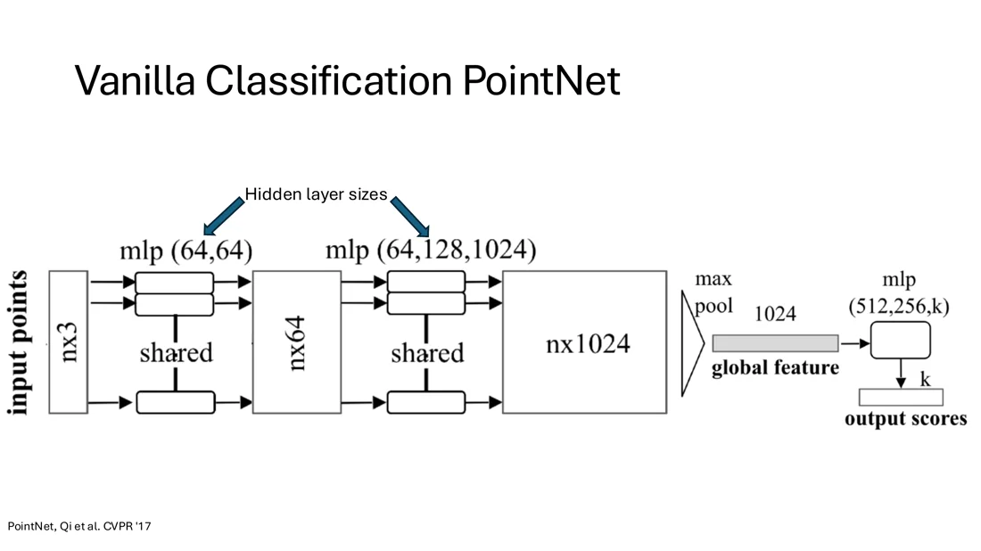
1. Start with an $n\times 3$ point cloud.
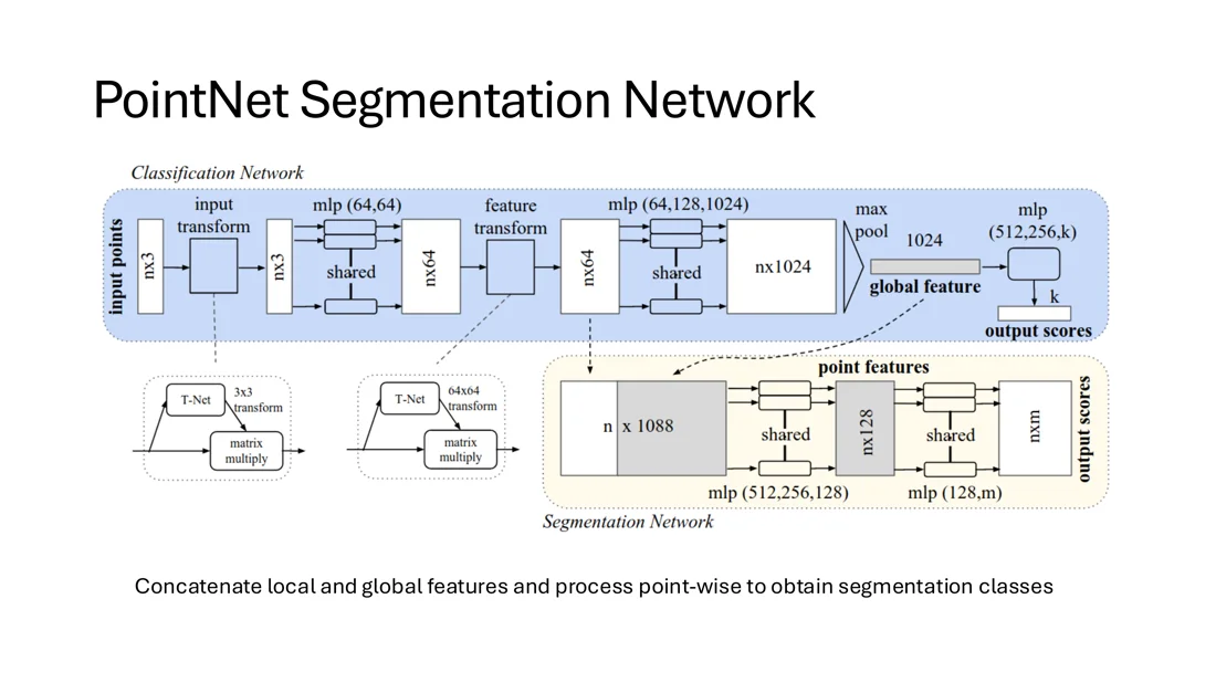
2. A shared MLP (64, 64) maps every point to a 64-dim vector → $n\times 64$. “Shared” means every point is processed by the same MLP with the same weights.
3. Another shared MLP (64, 128, 1024) → $n\times 1024$, one feature vector per point.
4. Max pooling → one global feature of size 1024.
5. An MLP (512, 256, $k$) → $k$ output scores (classes).

With max pooling, isn't only a single point relevant for the global feature?

Answer channel-wise: each of the 1024 channels can take its maximum from a different point.

No. Max pooling is done

Trap

“mlp(64, 64)” are two layers: $3\to 64$ (weights $3\times 64$), then $64\to 64$. Both are applied independently to each of the $N$ points, so there is no dimension mismatch.

Rotation Invariance: T-Nets

Slides 17-18

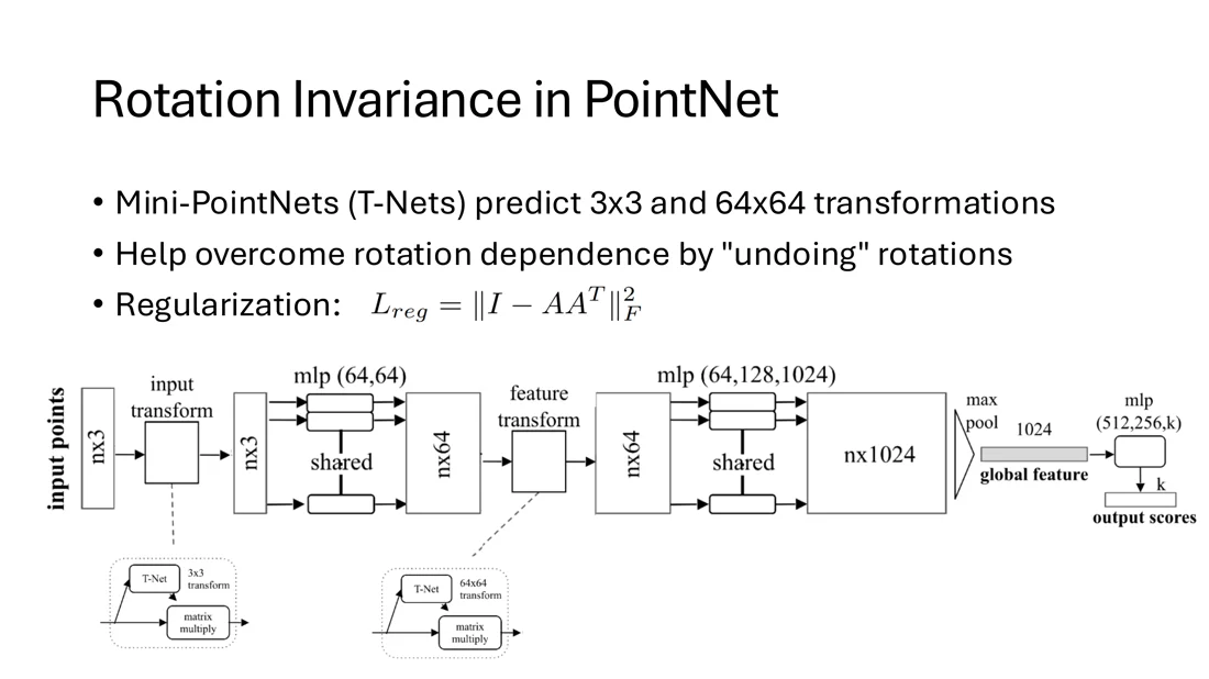
If we rotate the object, we expect the same output from the network. PointNet uses mini-PointNets (T-Nets) that predict a $3\times 3$ (input) and a $64\times 64$ (feature) transformation matrix. They help to overcome rotation dependence by “undoing” rotations. The feature transform is regularized to stay close to orthogonal:

T-Net regularization

$$L_{reg}=\Vert I-A{A}^T{\Vert }_F^2$$

$A$: the predicted feature transformation matrix.

Slide 18: T-Nets for the input and feature transforms.

Trap

T-Nets help, but they don’t guarantee rotation invariance. They don’t break permutation invariance.

Segmentation with PointNet

Slides 19-22

PointNet produces point-wise local features ($n\times 64$) and a global feature (1024). For segmentation we need both: concatenate the global feature to every point’s local feature ($n\times 1088$), and process point-wise with shared MLPs (512, 256, 128) and (128, $m$) → $n\times m$ scores.

Slide 20: PointNet segmentation network.

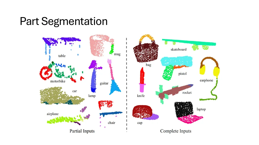
• Part segmentation: works on partial and complete inputs (table, mug, motorbike, …).
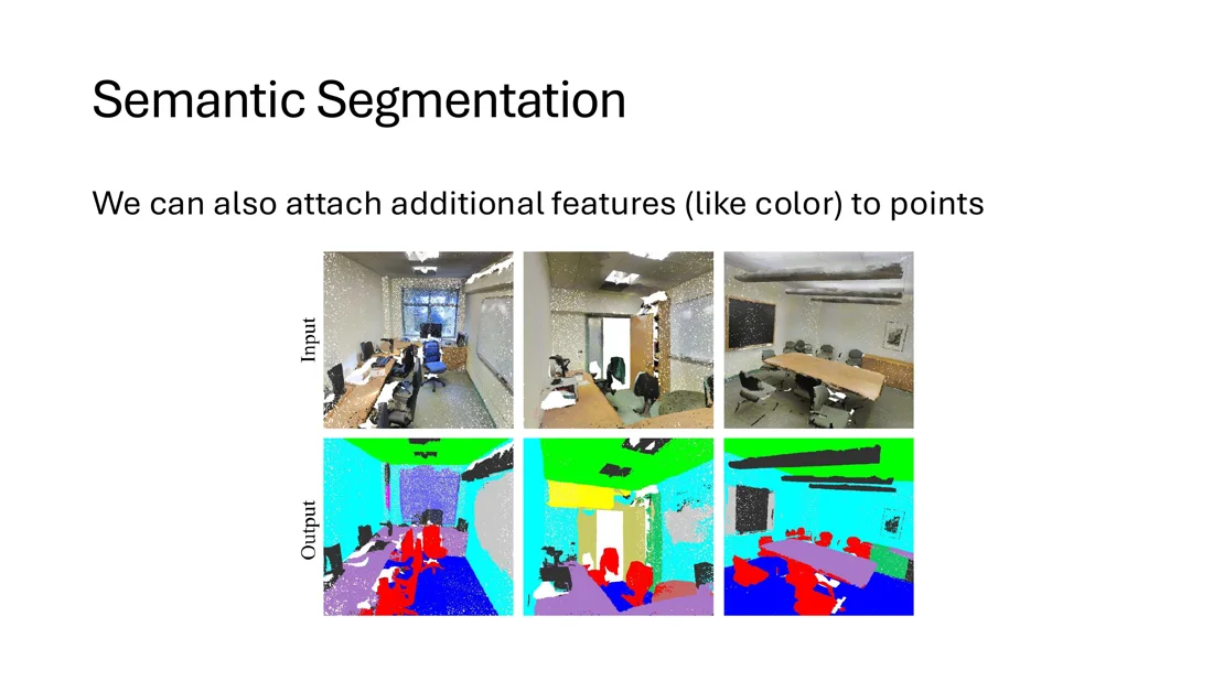
• Semantic segmentation: additional features can be attached to the points, e.g. 9-dim input: $(x,y,z)$, RGB, and the normalized location in the room.

Slide 21: part segmentation

Slide 22: semantic segmentation

PointNet++

CNN vs. PointNet: Locality

Slides 23-24

PointNet	CNN
per-point features + one global feature	progressively captures features at increasingly large scales
no notion of locality	multi-resolution hierarchy with increasing receptive fields

PointNet++ (Qi et al., NeurIPS 2017): a hierarchical network that exploits locality and uses PointNet as its basic block.

Hierarchical Point Set Feature Learning

Slides 25-27

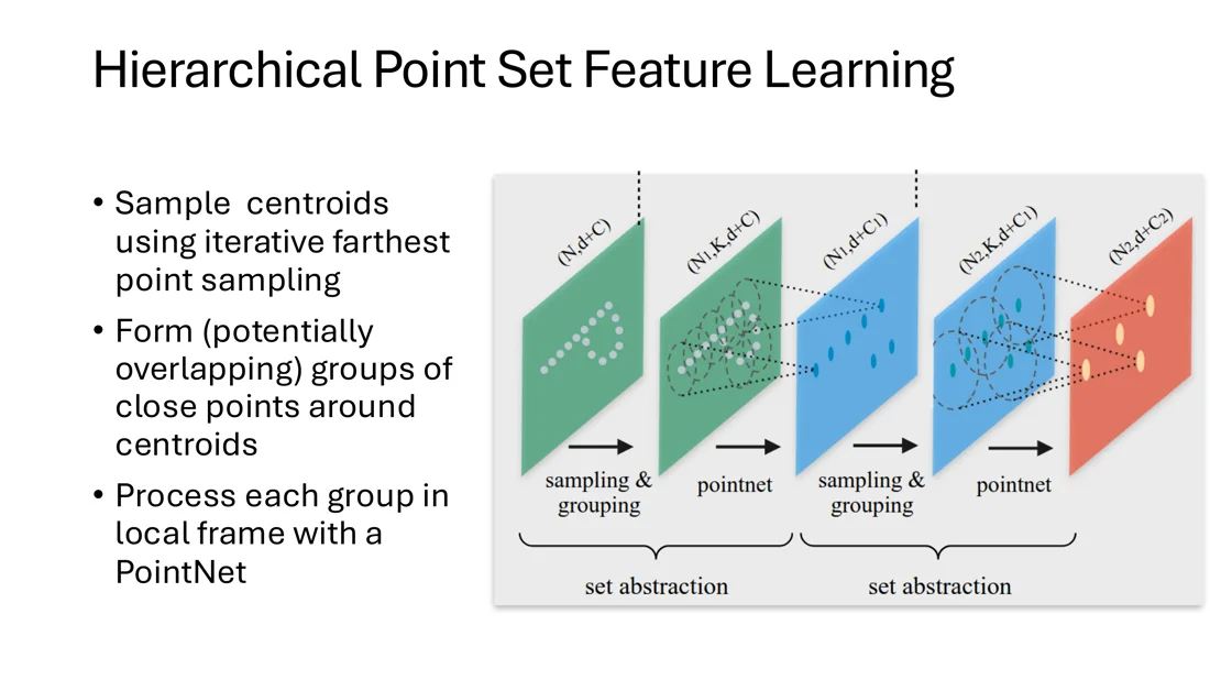
PointNet++ stacks several set abstraction levels. Each level processes a set of points and abstracts it into a new set with fewer elements but more features about the local neighborhood.

Set abstraction level

1. Sampling: sample centroids with iterative farthest point sampling (FPS), better than random.
2. Grouping: form (potentially overlapping) groups of close points around the centroids.
3. PointNet: process each group in its local frame (points translated relative to the centroid) with a PointNet.

$(N,d+C)\to (N_1,K,d+C)\to (N_1,d+C_1)$: $N_1$ centroids, $K$ points per group, $d=3$ coordinates, $C$ features.

Slide 26: hierarchical point set feature learning.

Intuition

Unlike in CNNs, the receptive fields are data-dependent. Groups may overlap, and the group scale can change from one layer to the next.

Classification: process the points and features of the final abstraction level with a PointNet and fully connected layers.

PointNet++ Segmentation: Feature Propagation

Slides 28-29

Problem: the original point set is subsampled, but we want a label for each original point. We only have features for the subsampled points.

Solution: feature propagation via interpolation. Propagate the features back level by level: interpolate the features of the $N_l$ points at the coordinates of the $N_{l-1}$ points (inverse distance weighted average over the $k=3$ nearest neighbors), concatenate them with the skip-linked features from the set abstraction level, and pass them through a “unit PointNet” (like a $1\times 1$ convolution). Repeat until we are back at the original points.

Slide 29: feature propagation with interpolation and skip links.

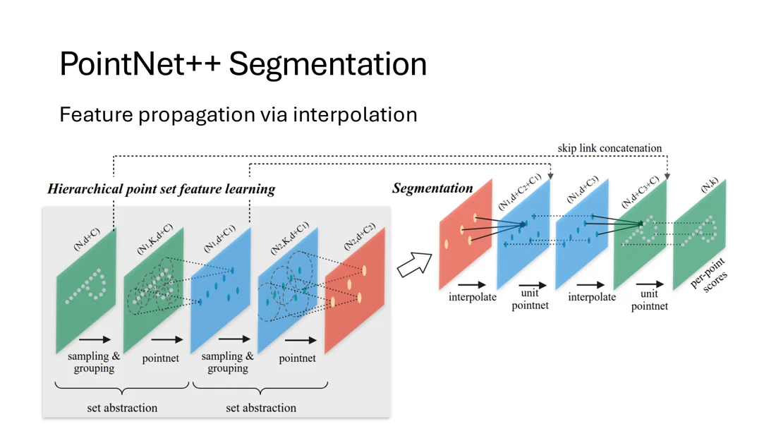
Summary (Slide 30): some improvement over vanilla PointNet (ModelNet40 accuracy 91.9% with normals vs. 89.2%), but increased complexity and more hyperparameters.

Trap

PointNet++ uses FPS, not random sampling; its groups overlap; there is no voxel grid. It does not replace PointNet, PointNet is its building block.

Transformers for Point Cloud Processing

Refresher: Attention

Slides 31-37

Attention was first used for translation: which source words matter for the next target word?

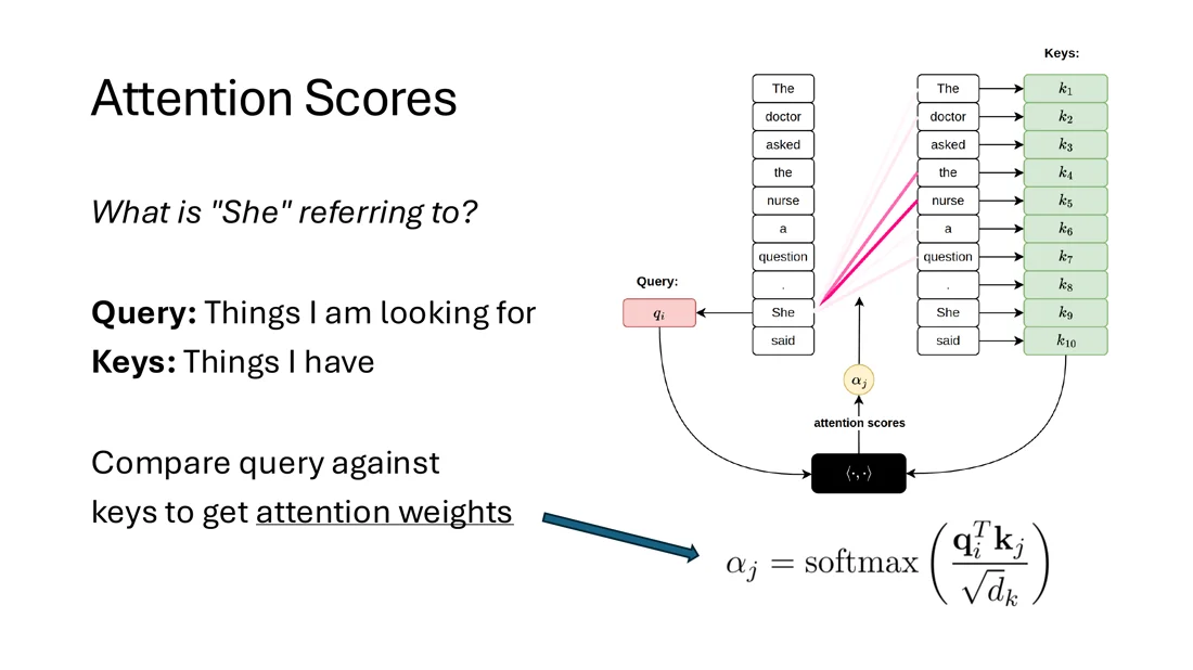
Query, key, value

Inspired by retrieval systems (e.g. a YouTube search):

• Query: the search query (things I am looking for)
• Keys: the video titles (things I have)
• Values: the videos (things I want to communicate)

Compare the query against the keys and return the values of the best matches.

Attention

Compare the query against the keys to get attention weights:

$${\alpha }_j=\text{softmax}\left(\frac{{\mathbf{q}}^T{\mathbf{k}}_j}{\sqrt{d_k}}\right)$$

Aggregate the values proportionally to the attention weights:

$$\mathbf{y}=\sum _j\text{softmax}\left(\frac{{\mathbf{q}}^T{\mathbf{k}}_j}{\sqrt{d_k}}\right){\mathbf{v}}_j$$

Slide 34: attention scores

Slide 35: value aggregation

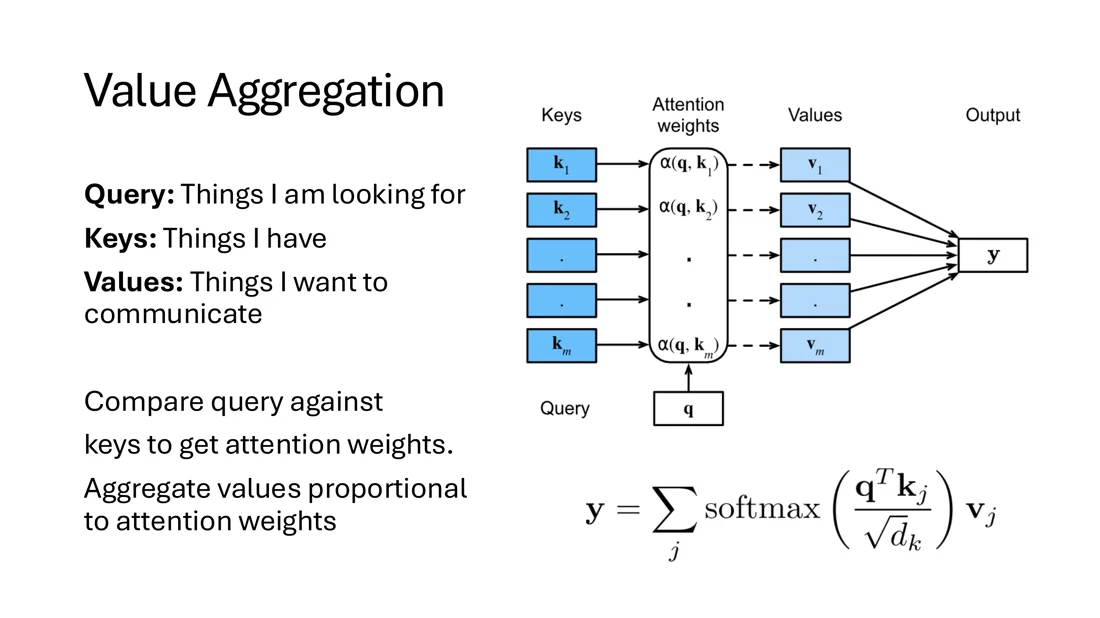
“Attention is all you need” (Vaswani et al., 2017) introduced the Transformer; the Vision Transformer applies it to image patches. In NLP and vision we need a positional encoding: numbers added to the tokens to indicate their position, because the tokens themselves carry no position.

Why transformers for point clouds? (Slide 38)

• extremely powerful for NLP and 2D vision
• naturally permutation-invariant (without a positional encoding)
• can process sequences of variable length

→ An ideal choice for point cloud processing.

Scalar vs. Vector Attention

Slides 39-40

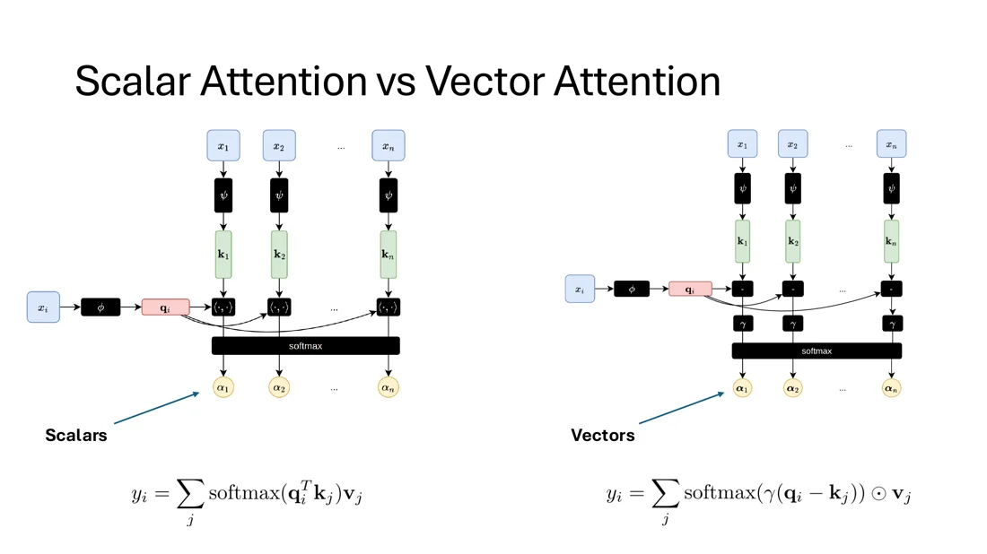
	Scalar attention	Vector attention
Formula	$y_i={\sum }_j\text{softmax}({\mathbf{q}}_i^T{\mathbf{k}}_j){\mathbf{v}}_j$	$y_i={\sum }_j\text{softmax}(\gamma ({\mathbf{q}}_i-{\mathbf{k}}_j))\odot {\mathbf{v}}_j$
Weights	one scalar per pair of points	a vector, same dimension as the value
Aggregation	linear combination of value vectors, all channels weighted the same	channel-wise (per-channel multiplication $\odot$)
Similarity	dot product	difference ${\mathbf{q}}_i-{\mathbf{k}}_j$, mapped by an MLP $\gamma$

(The scaling by $\sqrt{d}$ is left out for simplicity. $\varphi$ and $\psi$ are the linear maps from a token to its query and key.)

Slide 40: scalar vs. vector attention.

Intuition

Different channels of the value vectors may need to be aggregated differently. With scalar attention that is impossible; vector attention keeps the channel dimension, so each channel can attend differently to the same point. Attention over all points costs $\mathcal{O}(N^2)$.

Point Transformer

Slides 41-44

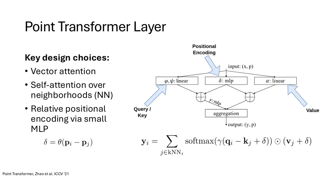
Point Transformer (Zhao et al., ICCV 2021). Key design choices:

1. vector attention
2. self-attention over local neighborhoods (the $k$ nearest neighbors)
3. relative positional encoding via a small MLP

Point Transformer layer

$${\mathbf{y}}_i=\sum _{j\in \text{kNN}(i)}\text{softmax}(\gamma ({\mathbf{q}}_i-{\mathbf{k}}_j+\delta ))\odot ({\mathbf{v}}_j+\delta ),\delta =\theta ({\mathbf{p}}_i-{\mathbf{p}}_j)$$

Input: points $\mathbf{p}$ with features $\mathbf{x}$. $\varphi ,\psi$ (linear): query and key; $\alpha$ (linear): value; $\gamma$ (MLP): attention weights; $\theta$ (MLP): positional encoding.

Slide 41: the point transformer layer.

Why a relative positional encoding?

In NLP, word tokens carry no position, so an absolute positional encoding is added to the tokens. Here every token is a 3D point, so the position is already there. The authors found it helpful to add the relative position to the neighbors, and it is added to both the attention and the value, not to the tokens.

Trap

On Slide 39, $\alpha$ denotes the attention weights; on Slide 41, $\alpha$ is the linear map that produces the values.

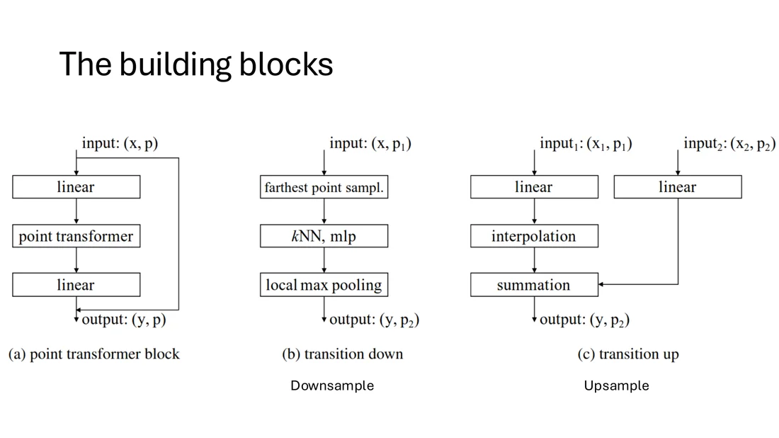
Building blocks (Slide 42):

• Point transformer block: linear → point transformer layer → linear, with a residual connection. Same number of points, new features.
• Transition down (downsample, similar to PointNet++ set abstraction): farthest point sampling, kNN + MLP, local max pooling.
• Transition up (upsample, for segmentation): linear, interpolation, summation with the skip-connected features.

Slide 42: the building blocks.

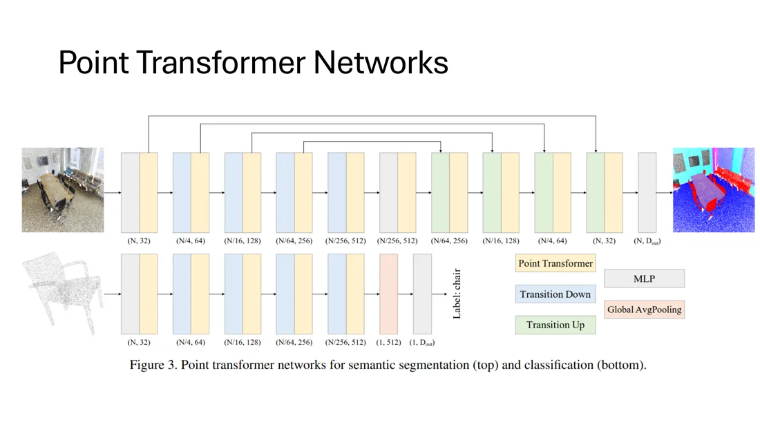
The segmentation network is a U-Net: an encoder of transition-down blocks and a decoder of transition-up blocks. The classification network is the encoder + global average pooling + an MLP.

Slide 43: Point Transformer networks.

Slide 44: semantic segmentation results.

Extensions

Slides 45-46

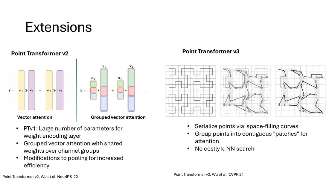
• Point Transformer v2 (Wu et al., NeurIPS 2022): in PTv1, the weight encoding layer gets a large number of parameters as the network gets deeper. PTv2 uses grouped vector attention with weights shared over groups of channels (more efficient, less overfitting), and modifies pooling for efficiency.
• Point Transformer v3 (Wu et al., CVPR 2024): serialize the points with space-filling curves, group them into contiguous “patches” for attention. No costly kNN search.
• Many more: OctFormer, PCT (Point Cloud Transformer), Swin3D, Superpoint Transformer, …

Slide 45: Point Transformer v2 and v3.

Summary

Slide 47

Method	Key idea	Solves
PointNet	shared MLP $h$ + symmetric $\max$ + MLP $f$	permutation invariance, variable number of points
PointNet++	FPS + grouping + PointNet per group, hierarchically	locality
Point Transformer	vector attention over kNN + relative positional encoding	expressive local aggregation

Self-Test

Why don't projection- and voxel-based approaches suffice?

Answer

Projection: 3D geometry is collapsed, sparsity is wasted, and the result depends on the chosen views. Voxels: geometric detail is lost by quantization unless the resolution (and memory) is very high.

Why doesn't sorting the points give permutation invariance?

Answer

A tiny perturbation can change the order drastically; no stable ordering exists in high dimensions.

Write down the vanilla PointNet and explain why it is permutation invariant.

Answer $f(g(h({\mathbf{x}}_1),\dots ,h({\mathbf{x}}_n)))$ with $h,f$ MLPs and $g=\max$. The shared $h$ is equivariant; the max is symmetric, so the result doesn't depend on the order. Max pooling also handles a variable number of points.

Does max pooling mean only one point determines the global feature?

Answer

No, it is channel-wise: each channel can come from a different point.

What do T-Nets do?

Answer $3\times 3$ input transform and a $64\times 64$ feature transform to undo rotations, regularized with $\Vert I-A{A}^T{\Vert }_F^2$. No guarantee of rotation invariance.

Mini-PointNets predict a

How does PointNet do segmentation?

Answer $n\times 1088$ and processes point-wise with shared MLPs.

It concatenates each point’s local feature (64) with the global feature (1024) to

Describe one set abstraction level of PointNet++.

Answer

Farthest point sampling of centroids, grouping (possibly overlapping) neighbors around them, a PointNet on each group in the local frame of its centroid.

How does PointNet++ get per-point labels?

Answer

Feature propagation: interpolate the features of the subsampled points back to the denser level (inverse distance weights, 3 nearest neighbors), concatenate skip-linked features, apply a unit PointNet, repeat.

What is the difference between scalar and vector attention?

Answer $\gamma ({\mathbf{q}}_i-{\mathbf{k}}_j)$ gives a weight vector, multiplied channel-wise with the values.

Scalar: one weight per pair (dot product), all channels weighted the same. Vector:

What are the three design choices of the Point Transformer?

Answer $\delta =\theta ({\mathbf{p}}_i-{\mathbf{p}}_j)$ added to the attention and the values.

Vector attention, self-attention over kNN neighborhoods, and a relative positional encoding

Related

• Previous: Lecture 6.1: Neural Fields · Next: Lecture 7: NeRF · Course: Overview
• Concepts: PointNet, Attention, Point Cloud, Voxel Grid
• IF-Nets (Lecture 6.1) are an alternative for point cloud inputs: voxelize, then 3D CNN features. Transformers come back in DUSt3R (Lecture 9).